Excel cell format means the background color, font color/style/size, number format, alignment, orientation, etc. attributes of a cell.
In this article, you will learn about Excel cell format.
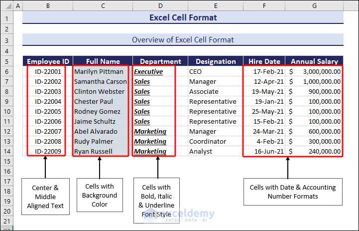
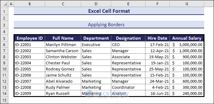
Here is an overview of formatting the cell text by changing its font style, size, and color.
In this article, you will learn:
– Excel cell format definition
– Options for formatting cells
– How to format cells with 14 examples
– Available number formats in Excel
– Solving number formatting issues
– Exclusive formatting options on the Format Cells dialog window
– Protecting cell format
– Shading cells
– Some useful shortcuts to format cells
– Copying cell format
– Clearing cell format
– Multiple text formatting in a single cell
– AutoFormat feature
In Excel, it’s often mandatory to format cell data or a range of data for user convenience. For example, an Excel formula may return a date as a whole number which in fact, makes no sense. So we need to change the format of that number to date so we can get meaningful results. Also, to make a cell unique from others, we may need to change the cell or font style and cell background color.
Note: While writing this article, we have used Excel for Microsoft 365, but you can also try these in other versions.
⏷ Excel Cell Format Definition
⏷ Options for Formatting Cells
⏷ How to Format Cells in Excel
⏷ Available Number Formats
⏷ Number Formatting Not Working
⏷ Use of Format Cells Dialog Window to Format Cell
⏷ Protection of Cell Format
⏷ Shading Cells in Excel
⏷ Some Useful Shortcuts to Format Cells
⏷ Copying Cell Format
⏷ Clearing Cell Format
⏷ Multiple Text Formatting in a Single Cell
⏷ AutoFormat Feature
What Is Excel Cell Format?
Cell formatting in Excel means making specific cells distinct and easy to read and understand.
For example, text data aligns to the left side of the cell and numeric data aligns to the right. The numeric data are in the General format by default.
Why do we need to format cells?- Look at the following image to understand this.
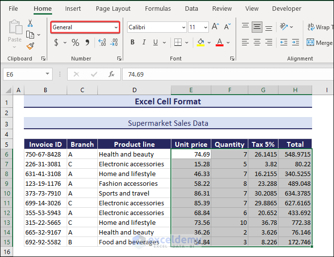
You can see that all the numeric data is in the General format. However, the Unit Price, Tax 5%, and Total columns are intended to display a $ symbol before them for a better understanding of the values.
Why Do We Need to Format Cells?
- Formatting cells make numbers and text easy on the eyes, avoiding confusion and making your data a breeze to go through.
- Adding $ signs or % symbols clarifies what the numbers represent, helping everyone understand at a glance.
- Use bold colors to point out what matters in your data, making it pop.
- Formatting maintains a clean, consistent look, making your spreadsheet look polished and professional.
- Well-formatted cells mean you spend less time figuring out what’s what and more time making decisions based on your data.
What Options Are Available to Format Cells in Excel?
1. Ribbon Commands
There are various commands in the Ribbon to format a cell in Excel. You can find options to format alignment, font, styles, numbers, etc. Here, I’m showing you some formatting options of the Number group.

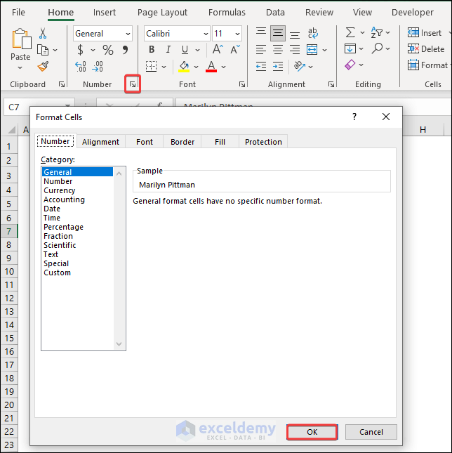
2. Commands on Format Cells Dialog
There are four ways we can use to open the cell formatting options, in other words, the Format Cells dialog box.
- Using Keyboard Shortcut
- Home ⇒ Format ⇒ Cells ⇒ Format Cells
- Right-Click ⇒ Format Cells command
- Home ⇒ Number group ⇒ click on the dialog box launcher.
How to Format Cells in Excel? – See 14 Examples
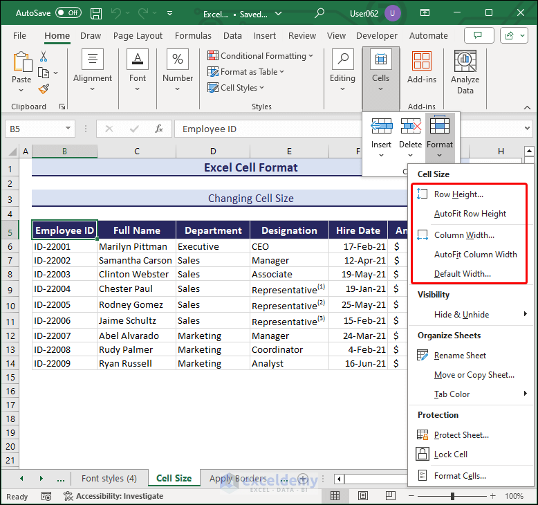
1. Changing Cell Size
To change the length of a cell or increase the column width, just drag the column width icon left or right to adjust. You need to drag the row up or down to increase or decrease its height. You can also double-click to adjust the height or width automatically.
Thus, all the data can be seen clearly after formatting the cell size.
You can also find the options for changing the cell size under the Format group in the ribbon. See the following image.
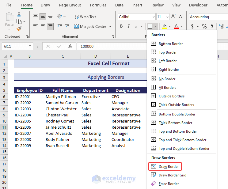
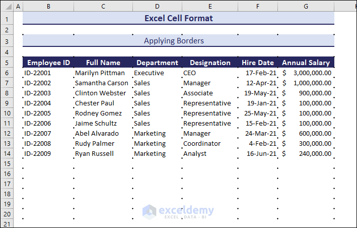
2. Applying Cell Borders
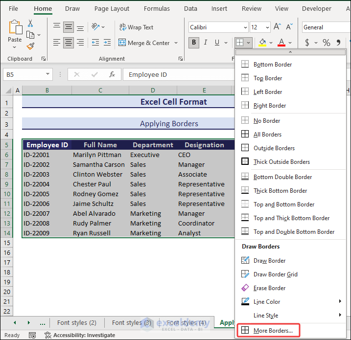
To apply borders to the data table, just select the data range and select All Borders under the Border drop-down. Follow the image below.
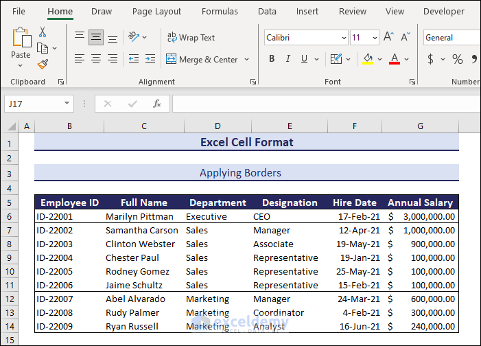
You can see that there are a lot of Border options in the drop-down menu. If you want to use the border around the data table only, you can use the Outside Border. See the below to get a better understanding.
There are other types of borders such as Top and Bottom borders, Left border, Right border, Thick Outside Borders, etc. which are rarely used.
Moreover, you can customize the border too. In that case, you can draw the border manually. To open this feature, select Draw Border under the Borders drop-down.
You will see dots at the edge of each cell. Connect them by using a mouse.
Select the Draw Border option from the Border drop-down again. The borders will be created and the dots will disappear. Or press Esc.
Note: There are some other features under the Draw Borders option.
- Draw Border Grid feature helps you to draw borders without dragging the cursor like the Draw Border
- Erase Border feature removes borders when necessary.
- The Line Color and Line Style features help to set up border colors and styles.
There is also an option for applying borders of different line styles. Say, you want solid lines for outside borders and dotted lines for inside borders. To create this type of border, you need to select the More Borders option first.
After that, the Format Cells dialog box will appear. Select the Border tab and choose the Line Styles and corresponding Border sides. You can see a preview of the border style in the Border section of the dialog box. You can also choose different colors for borders if you want.
In the image below,
The Line Styles for the outside border are marked by red rectangles.
For inside borders, line styles for inside borders are marked dark blue.
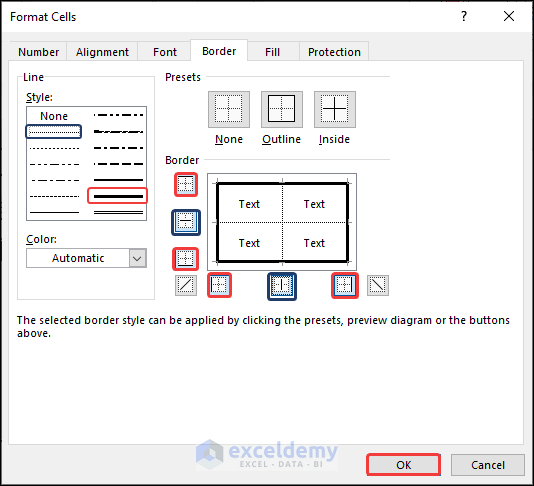
After clicking OK, you will see the desired border style in the data table.
Thus you can apply borders to format cells.
Note: To remove the border from a cell or range of cells, select them and use the No Border command from the border drop-down. Or you can press Ctrl + Shift + –.
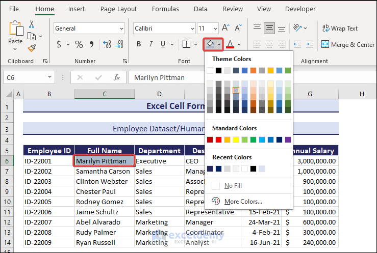
3. Changing Cell Background Color
By default, an Excel cell in No Fill background format. To change the cell color to another color-
Select the cell ⇒ go to Home ⇒ Font group of commands ⇒ open the Fill Color menu and choose a color.
4. Changing Font Type, Font Size, and Font Color
You will find the commands to change font type, style, size, and color in the Font group of the Home tab under the Excel ribbon.
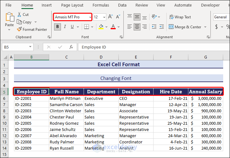
4.1 Changing Font Type
To change the font of the text, select the cell or the range of cells and choose a font of your preference from the Font drop-down.
Here, we set the font of the column headers to Amasis MT Pro.
4.2 Changing Font Size
We can also increase or decrease the font size from the Font Size drop-down in the Font group.
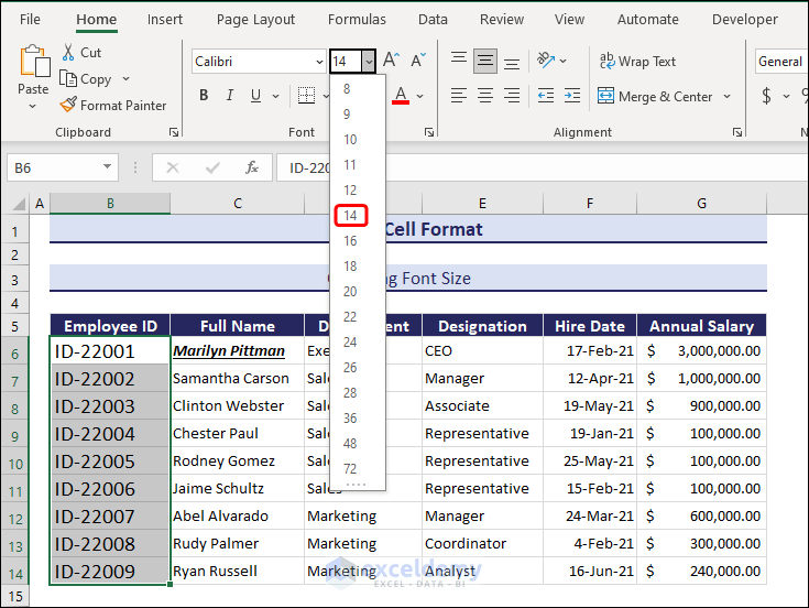
In the image above, the IDs are sized to 14.
You can apply any size (including fractional numbers) by typing manually in the Font Size box.
The Font group also has 2 buttons to increase and decrease the font size. Follow the image below to see the procedure.
Note: Font size can also be changed using a keyboard shortcut. Just select the cell and press Alt + H + F + G to increase the font size. To decrease the size, press Alt + H + F + K.
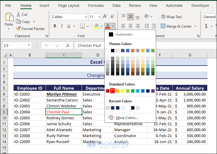
4.3 Changing Font Color
Say, Chester Paul, an employee failed to achieve his work target. You want to mark his name with a red color font.
To do that, select his name and open the drop-down of the Font Color
Choose the Red color and you will see the name font is red.
5. Making Cell Content Bold, Italic, and Underlined
We can apply 3 different styles to the font of a text. These are: Bold, Italic, and Underline. You can find these styles in the Font group. Whenever you need to change a font style, just click the corresponding button.
Here, we applied these styles to the text in cell C6.
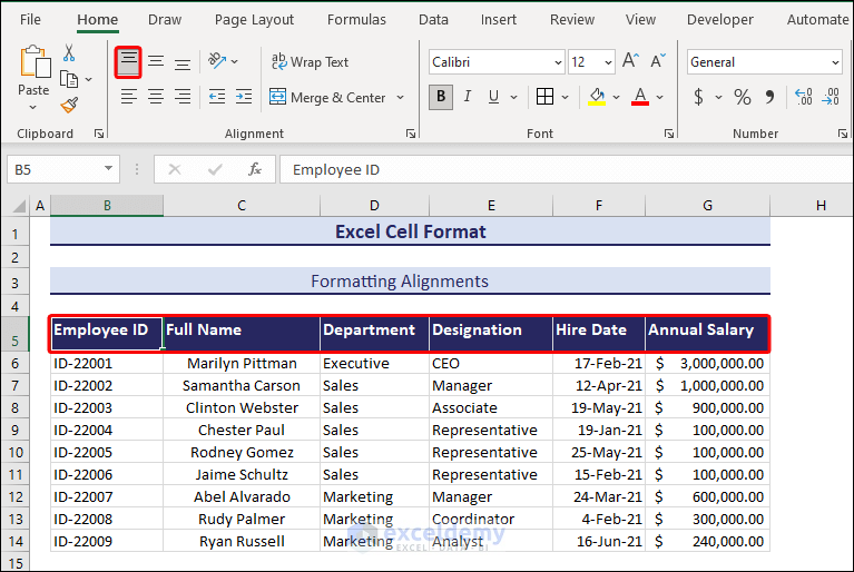
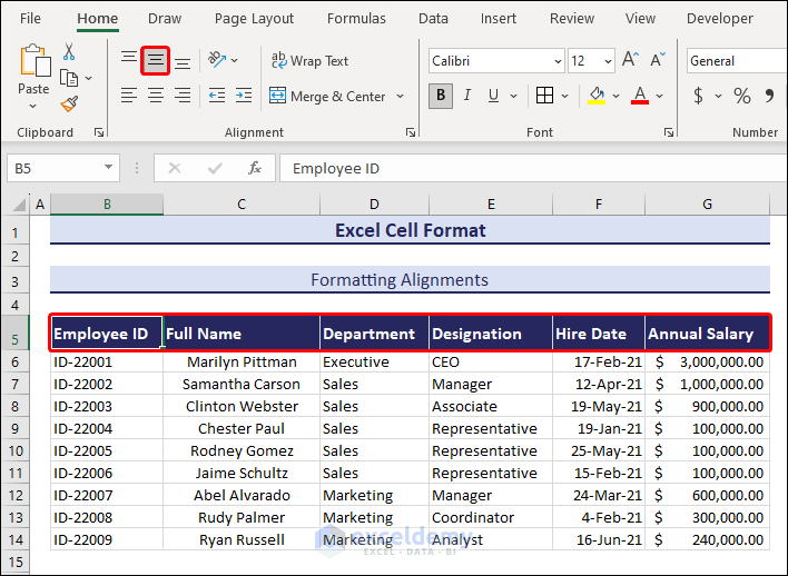
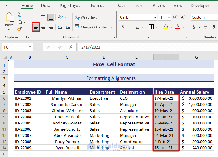
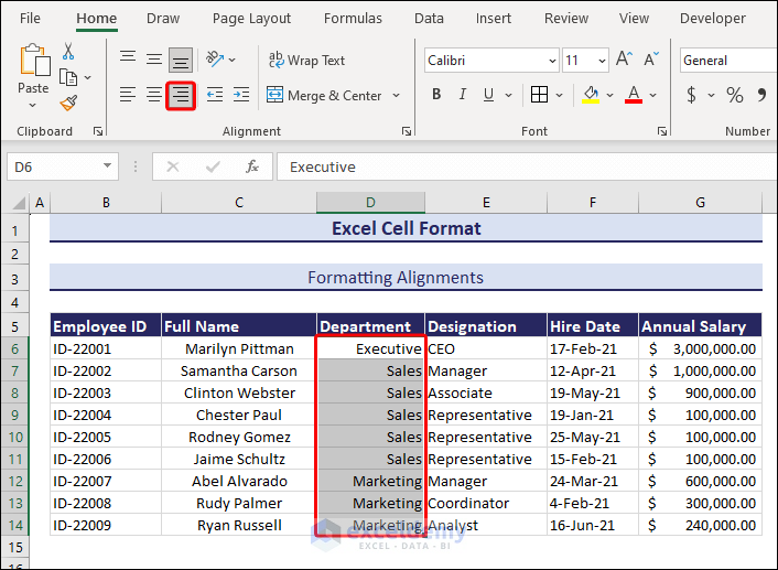
6. Changing the Alignment of Cell Contents
Normally, text data stays at the left side of the cell and numeric data falls to the right when inserted in an Excel cell. This is the default alignment of the data. But there are options in the Alignment group of ribbons to change this alignment.
In the following image, I’ve shown you the Center and Middle alignments on the Full Name column.
You can see that there are more alignment options in the Alignment group. Excel has two types of alignments: Horizontal and Vertical. Both of them are divided into different classes. I’ll be showing them in the following section.
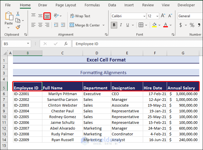
Top alignment feature moves the cell contents to the top of a cell.
Middle alignment keeps the cell contents in the middle of a cell.
Bottom alignment moves the cell contents to the bottom of a cell.
Center alignment keeps the cell contents in the center position of a cell.
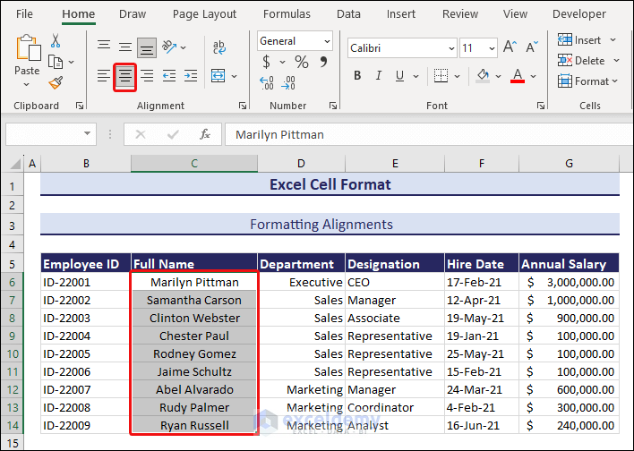
Left alignment moves the cell contents to the left of a cell.
Right alignment moves the cell contents to the right of a cell.
7. Increasing or Decreasing Cell Indent
Indent is a formatting feature in Excel that lets the users move any data within a cell by changing the indent. In the following image, we have shown how to indent data in a cell.
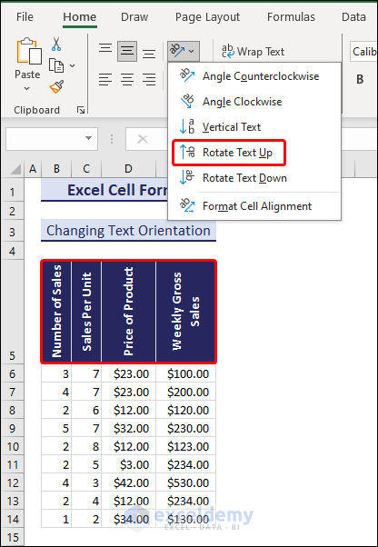
8. Changing Text Orientation Inside Cells
Sometimes we may need to change the orientation of data for a different view of the data table or to save spaces.
To apply text orientation on a set of cells, you need to select them first and then choose any of the orientation options of your preference under the Orientation drop-down.
The following image shows that the columns are wide due to the headers, while the data under the header are narrower.
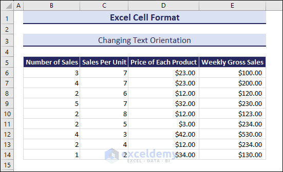
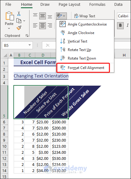
That’s why, I applied Angle Counterclockwise orientation from the Alignment ribbon section to the range B5:E5. Follow the image below to understand the procedure.
To use custom orientation, select the B5:E5 range first.
After that, select the Format Cell Alignment option under the Orientation drop-down or press Ctrl + 1 to open the Format Cells dialog box.
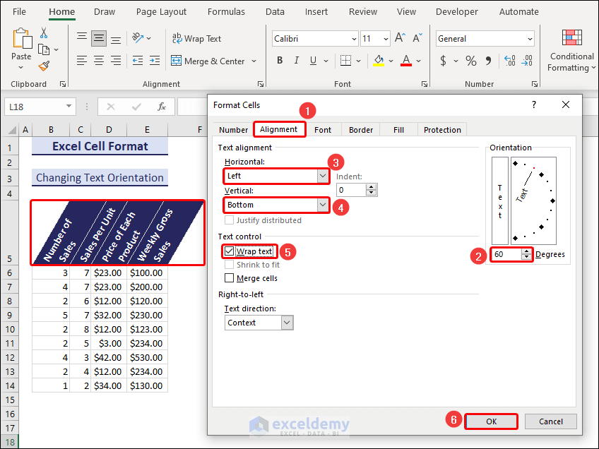
Next, set an angle for the Orientations under the Alignment
After that, set up the Horizontal and Vertical Text Alignments according to your preference.
Thereafter, select a Text control Here I chose Wrap text. Then we click OK to execute the commands.
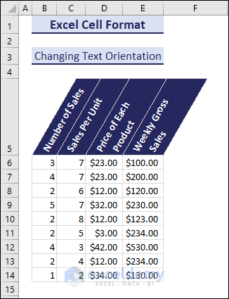
You can see the custom-oriented texts in the following image.
You can also rotate the text 90 degrees. For this purpose, I use the Rotate Text Up It can be useful to save space.
9. Wrapping Text in a Cell
Here, the names of the employees are not fully visible. We can use the Wrap Text command to fix the problem without making the column width bigger.
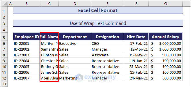
To apply the command correctly, select the cell range (B5:B12).
Next, select the Wrap Text command and autofit the column width if needed.
10. Merging Cells
Here, I’m giving a title to the data table. The title is on the top left corner of the table.

To put the title on the center top of the data table, use the Merge & Center command from the Alignment group.
You may apply a background color if you want in the merged cells.
11. Applying Default Cell Styles or Create New
In this section, we formatted the column headings using the default Cell Style employed by Excel.
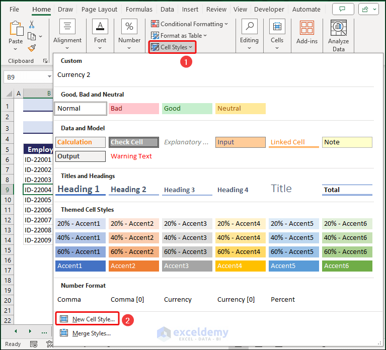
To insert a cell style format, select the cell or range of cells, and then go to Home ⇒ Cell Styles drop-down and choose the style you want.
To create a custom style, select New Cell Style from the Cell Styles drop-down.
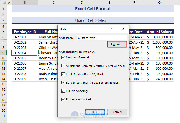
The Style dialog box will appear. Provide a Style name and click the Format… button.
Check or uncheck the Style includes parameters.
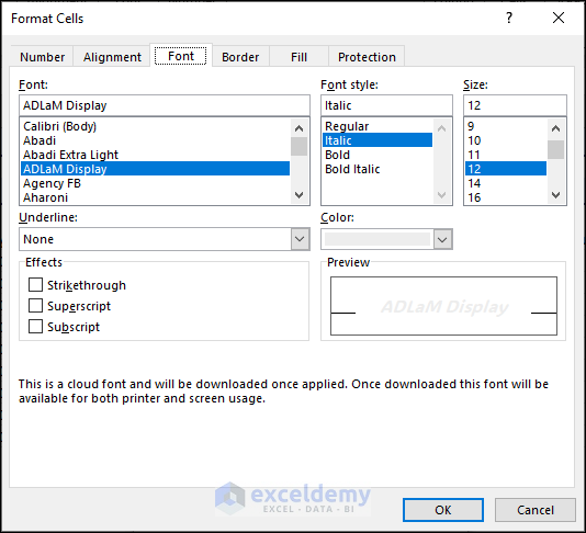
The Format Cells dialog box will appear. Navigate to the tabs and choose your formatting. Here, I will format the Font and Fill
The following picture shows the Font, Font Color, Font Style, and Size of the font that I chose.
And here I applied a Fill background color to the column headings. I also select a Pattern Color and Style to make the header a unique look.
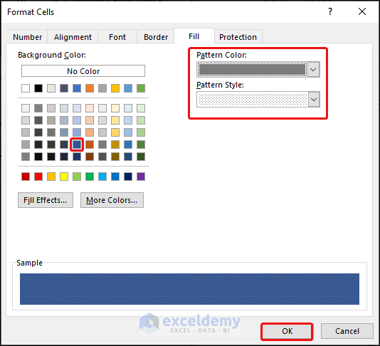
After clicking OK, you can see that the name of the Custom Style appears under the Cell Styles drop-down. Select it for the headers and you can see the style applied.
If you want to remove the style, just select the styled cells and choose Normal under the Cell Styles drop-down.
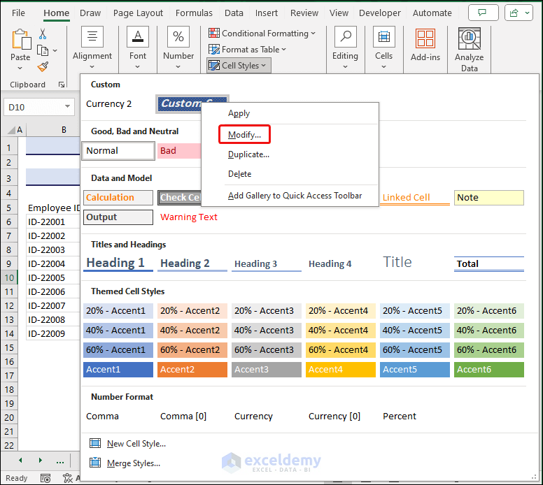
If you want to edit the Custom style, you can open the styles from the Styles drop-down, right-click on the Custom Style, and select Modify from the Context Menu.
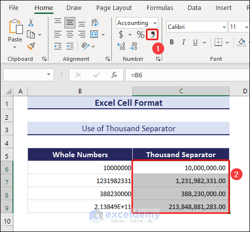
12. Use of Thousand Separators in Numbers
Here, I have used thousand separators for some large and whole numbers. You can find the Thousands Separator button in the Number group.
13. Increasing or Decreasing Decimal Places
You can change the decimal places by selecting the buttons for increasing or decreasing decimal places in the Number group. See the image below.
14. Changing Number Formats
Excel can recognize the following data types when you write them in a proper format: number, text, date, time, and percentage. However, we can format them according to our preferences. The upcoming sections will show a detailed description
What Are the Available Number Formats in Excel?
In the following image, you can see the number formats available in Excel. We will have a short explanation for each of them later.
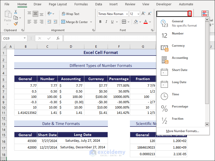
As you can see, there are 12 default formats available in Excel. Additionally, you can modify the custom format based on your data. When we do cell formatting, most of the time it refers to formatting the numbers.
Go through the table below to get a basic idea of them. Later, we’ll show some examples with images.
| Format | Description |
|---|---|
| General | When you type a number into Excel, it uses the default number format. Numbers typed with the General format are often displayed exactly as you input them. If the cell is too small to display the complete number, the General format rounds the numbers with decimals. For large numbers (12 or more digits), the General number format additionally employs scientific (exponential) notation. |
| Number | Used to display numbers in general with decimals. You can choose the number of decimal places to display, whether to use a thousand separator, and how to display negative integers. |
| Currency | Used for showing values with the default currency symbol. You can specify the number of decimal places that you want to use, whether you want to use a thousand separator, and how you want to display negative numbers. |
| Accounting | We also use it for monetary values, however, it aligns currency symbols and decimal points in a column. |
| Date | Date and time serial numbers are displayed as date values according to the locale (place) that you pick. Date formats that begin with an asterisk (*) respond to changes in the Control Panel’s regional date and time settings. Control Panel adjustments do not affect formats denoted by an asterisk. |
| Time | The functionality of this format is similar to the Date format. It just displays date and time serial numbers as time values. |
| Percentage | The cell value is multiplied by 100, and the result is displayed with a percent (%) sign. You can define the number of decimal places to be used. |
| Fraction | Displays a number as a fraction based on the fraction type you provide. |
| Scientific | Displays a number in exponential notation, replacing part of it with E+n, where E (Exponent) multiplies the preceding number by 10 to the nth power. A 2-decimal Scientific format, for example, displays 276384772367 as 2.76E+10, which is 2.76 times 10 to the 10th power. You can define the number of decimal places to be used. |
| Text | Treats cell content as text and displays it precisely as you input it, even when you type numbers. |
| Special | Can be used to represent a number as a postal code (ZIP Code), phone number, or Social Security number. |
| Custom | You can change a copy of an existing number format code. This format is used to add a custom number format to the list of number format codes. Depending on the language version of Excel installed on your computer, you can add between 200 and 250 special number formats. |
When you insert a number in a cell, Excel displays it in its default form. This number is treated as General by Excel.
The following image shows different number formats like Number, Accounting, Currency, Percentage, Fraction, and Text for the numbers in column B. Also, you will see more number formats, such as Short Date, Long Date, Time, and Scientific.
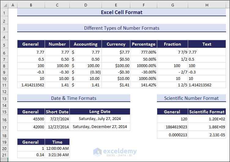
You can apply these formats from the Number drop-down. To apply these formats, you just have to select the range of cells containing numbers and select a suitable format from the drop-down.
These are the default number formats employed by Excel.
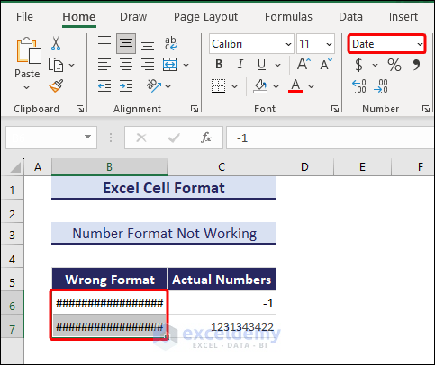
Number Formatting Not Working in Excel? – Let’s Troubleshoot
Sometimes, you may see a series of hash symbols (#) while entering a number in a cell. This may happen because of improper formatting of the cell.
For instance, if your cell is formatted to date but you enter a negative number, you will face this problem.
You may also notice that there is another issue with the number in cell J6. This number is formatted to date but exceeds the serial number a date can store. The highest date in Excel is 12/31/9999 which is recognized as 2958465 by Excel.
You may also see the hash symbols if the numbers don’t fit in a cell completely. In that case, just increase the column width.
How to Use the Format Cells Dialog Window to Format Cells in Excel?
Some formatting options are not available in the ribbon but you can get them in the Format Cells dialog box.
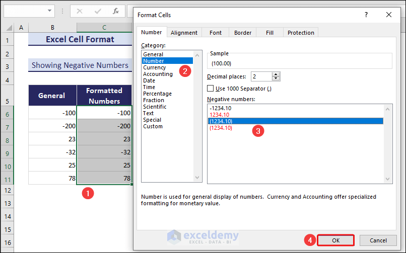
1. Displaying Negative Numbers
Sometimes, users prefer to express negative numbers differently. Sometimes it’s better to show negative numbers differently so the user can understand that there is a decrease in the data, especially in accounting.
Here are some default options to show negative numbers.
- Here, we have selected some numbers and navigated to the Number option of the Format Cells dialog box.
- After that, we selected one of the four Negative number formats and clicked OK.
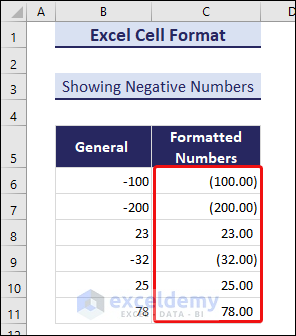
Here are the formatted negative numbers.
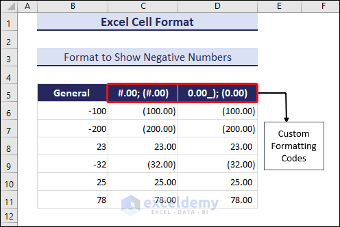
Moreover, the codes below are also for formatting negative numbers.
Codes:
- #.00; (#.00)
- 00_); (0.00)
Note: To see how to use the codes in the Format Cells dialog box, follow the process shown in the Customizing Number Format section.
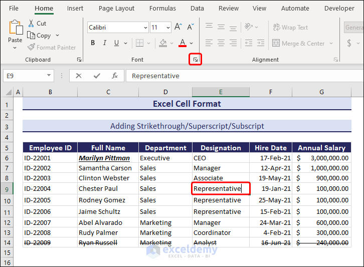
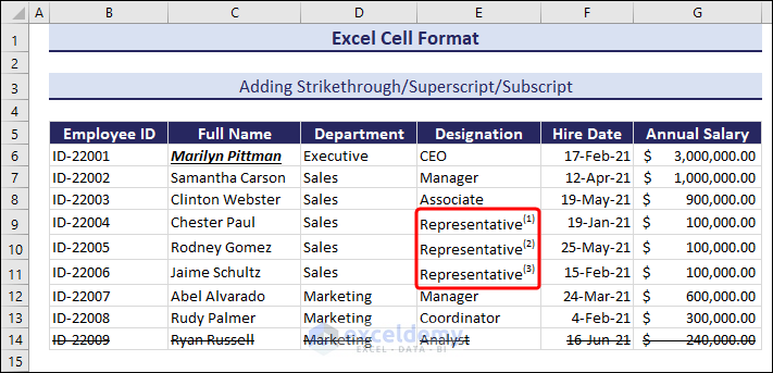
2. Adding Strikethrough/Superscript/Subscript
Strikethrough means a line through the text in a cell. If something is excluded or finished from your dataset but you want to keep the record in the sheet, you can use a Strikethrough for that purpose.
Say, the employee Ryan Russell resigned from the company. We are going to apply Strikethrough in the row where his entries are stored.
- To put the Strikethrough in the row, select the range of cells and press Ctrl + 1 or click the dialog box launcher in the Font group to open the Format Cells dialog box.
- Next, check Strikethrough and click OK. Make sure you select the Font tab of the Format Cells window.
Now, I’m going to show an example of using the Superscript feature. Say, I want to mark the Representative employees by Representative(1), Representative(2), and Representative(3).
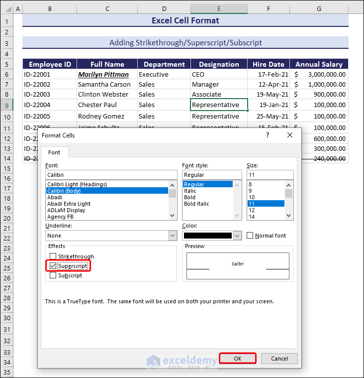
- To use Superscript in a cell, first double-click on that cell to go to the edit mode.
- Now, click the dialog box launcher of the Font group.
- The Font tab of the Format Cells window will appear.
- Check Superscript and click OK.
- Now, type the number as we showed earlier. You will see the number as Superscript to the text.
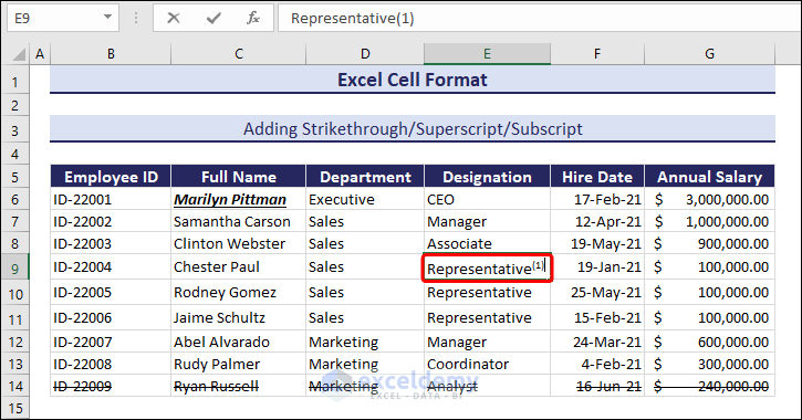
- Press Enter and apply the procedure to the other “Representative” Or you can copy the data and replace 1 with 2 and 3 respectively.
You can add a Subscript to a text in the same way.
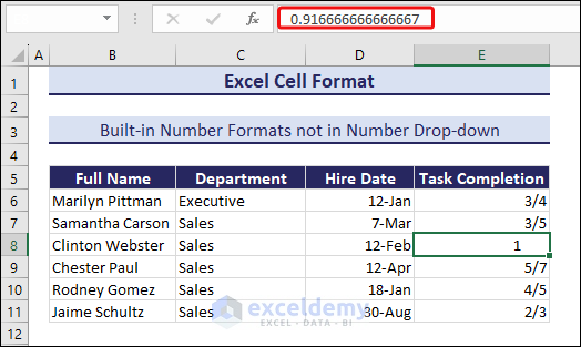
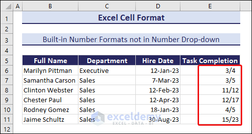
3. Some Built-in Number Formats That Are Not Available in Number Drop-down
Some built-in number formats are not available in the ribbon. I will show you some of them with applications.
The following image shows the date and fraction formatted numbers. I want to add the years to dates and make the fractions more precise as the default format returns approximate values up to 1 digit.
To format the dates,
- Select them and press Ctrl + 1 to open the Format Cells
- Next, select Date ⇒ Type ⇒ type of date format containing year (14-Mar-12).

Click on the image to enlarge
After clicking OK, the years will be added to the dates.
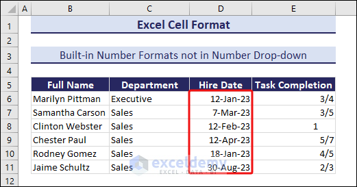
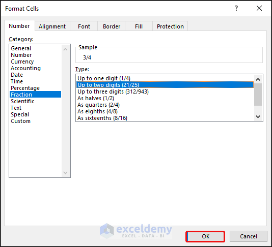
- To format the factional numbers, similarly select them and open the Format Cells
- After that, select Fraction ⇒ Up to two digits (21/25). You may also choose the Up to three digits option for better precision.
After clicking OK, the fractions will have a more precise format.
These are some built-in number formats that are not available in the ribbon list.
4. Customizing Number Formats
We commonly use some units such as kilometers, kilograms, degrees Celsius, inches, centimeters, etc. But normally we cannot use those units in the numeric data. Here, I’ll show you how you can format numeric data to such units using the Custom Format feature.
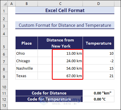
Here, I have some distances between two places and the temperatures of the places. To convert numbers to km (kilometer) units, use the following code for the data range.
Code:
0.00 “km”
To convert numbers to degree Celsius units, use the following code:
0.00 °C
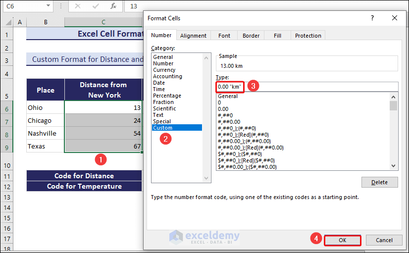
To format the distances with kilometers units,
- First, select the range of numbers.
- Open the Format Cells dialog box by pressing Ctrl + 1.
- Select Custom >> Type the code 00 “km” in the Type section.
- Click OK.
You can see the numbers converted to the kilometer units next.
- Similarly, insert the code for degree Celsius units in the Format Cells dialog box.
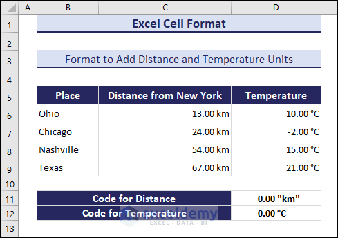
Thus you can customize number formats to present numeric data in any form.
How to Protect Cell Format in Excel?
By default, all the cells in Excel are locked, although it doesn’t have any effect unless you protect the sheet. If you don’t want to lose the formatting in a sheet, you need to protect the sheet. For this purpose,
- Select Format ⇒ Protect Sheet.
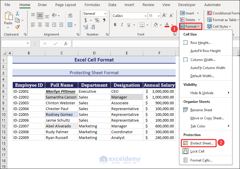
- Next, in the Protect Sheet dialog box, insert a password and check the following options shown in the image below.
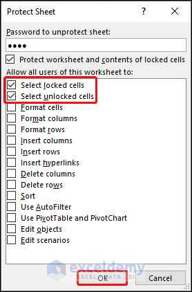
- Reenter the password in the next pop-up window and you will see the formatting features are grayed out. No one will be able to make any changes to the sheet. If someone does, a warning message will be delivered.

Click on the image to enlarge
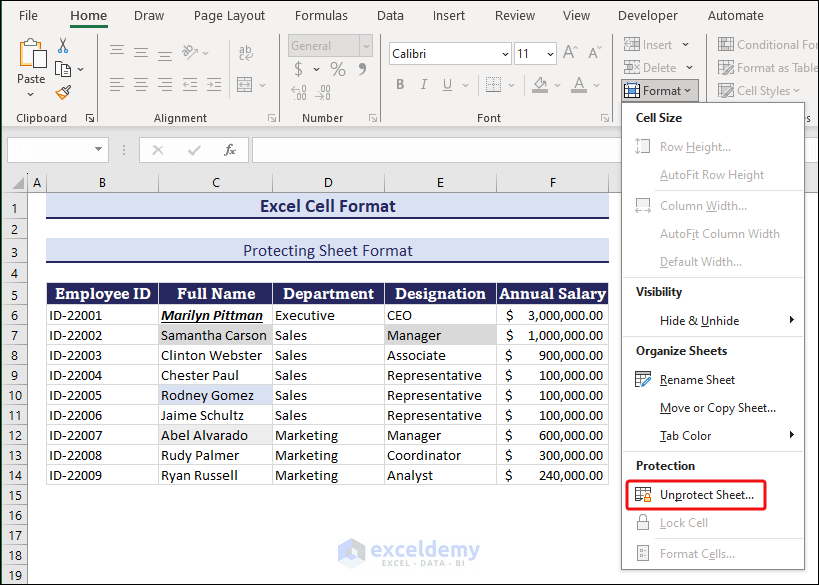
To enable formatting in the sheet, simply unprotect it with the password.
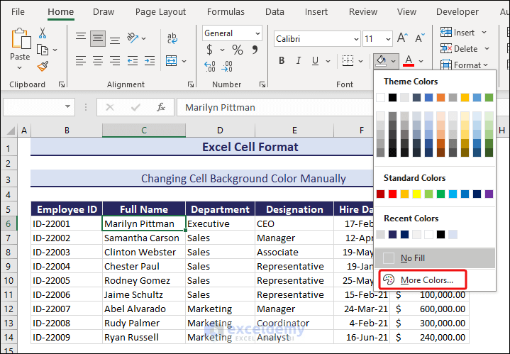
How to Shade Cells in Excel?
Shading a cell means inserting a background color to that cell and applying some effects or pattern color. We have already seen how to insert background color in a cell. So let’s learn some new tricks for formatting cells.
- Select the cell you want to shade and open More Colors options from the Fill Color drop-down. Here, I’ll shade the C6 cell.
- After that, the Colors dialog box will pop up.
- You will find some default colors in the Standard However, I want to make a custom color. So I selected the Custom tab and dragged the marked icons in the image to create a new color.
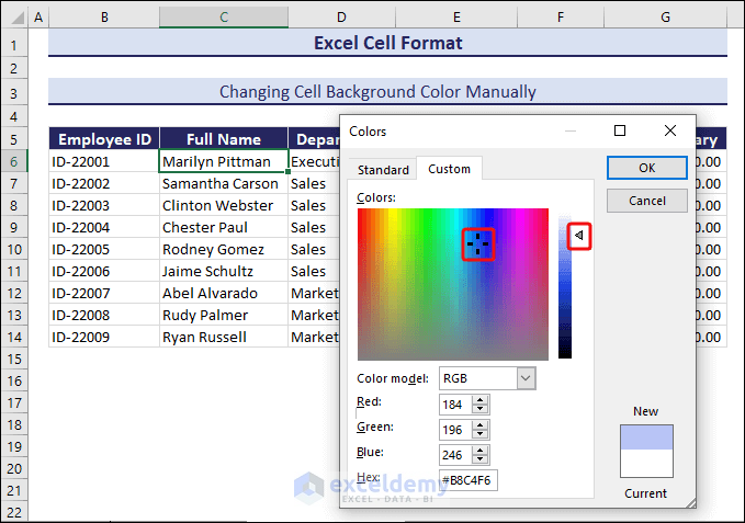
You can see the color under the New portion. Click OK to continue. We are going to insert some color effects to provide shading in the cell.
- Next, the background color will be applied to the cell.
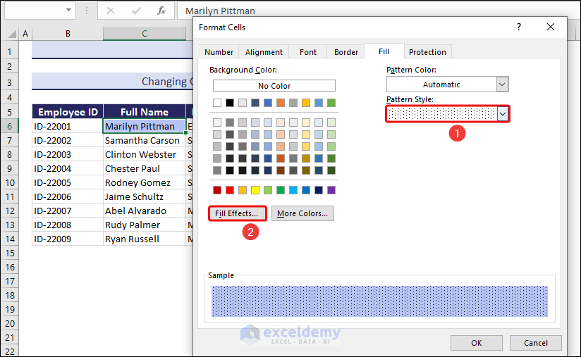
- Keep the cell selected and press Ctrl + 1 to open the Format Cells dialog box.
- After that, select Fill >> apply a Pattern Style >> click the Fill Effects…
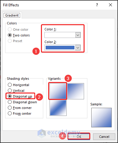
- The Fill Effects dialog box will pop up.
- Select Two colors >> Color 1 and Color 3 according to your preference.
- After that, choose one of the Shading styles.
- Here, I select the Diagonal up style and then choose the 1st Variant.
- Next, click the OK button in the Fill Effects and Format Cells dialog box one after another.
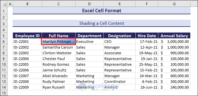
Finally, you will see the content of the cell C6 shaded.
Some Useful Shortcuts to Format Cells in Excel
Here is a list of useful keyboard shortcuts that may ease up your formatting task.
| Keyboard Shortcuts | Output |
|---|---|
| Ctrl + Shift + ~ | Returns General format |
| Ctrl + Shift + % or 5 | Returns Percentage format |
| Ctrl + Shift + $ or 4 | Returns Currency format |
| Ctrl + Shift + ^ or 6 | Returns Scientific format |
| Ctrl + Shift + ! or 1 | Returns Number format |
| Ctrl + Shift + # | Returns Date format |
| Ctrl + Shift + @ | Returns Time format |
| Ctrl + B | Returns or removes Bold format |
| Ctrl + I | Returns or removes Italic format |
| Ctrl + U | Returns or removes Underline format |
| Ctrl + 5 | Returns or removes Strike format |
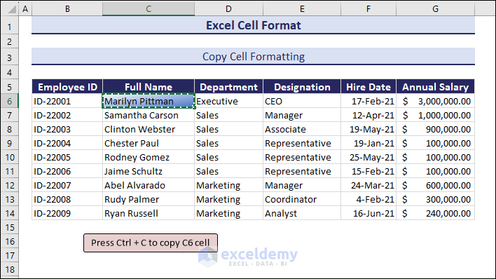
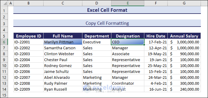
How to Copy Cell Format in Excel?
There are multiple ways to copy cell format in Excel: using the Format Painter tool, using the Paste Formatting command from the Right-Click menu appearing after a cell is copied, and Paste Special dialog box.
You can only apply the formatting of one cell to another or multiple cells by using the Copy Formatting feature.
- Say, we want to copy the formatting of cell C6 to C8. For this purpose, you need to select a cell with data and formatting, then press Ctrl + C to copy it.
- Now, right-click on the cell you want the formatting to be copied and select Paste Options >> Formatting Icon. Follow the image below for clarification.
After that, you will see that the formatting is copied only on C8.
This can also be done for multiple cells. Just select a range of cells before pasting the format.
There is another way of copying the format of a cell to another. This is known as the Format Painter feature. Say, you want the E6 cell to have the formatting of cell C6.
- To apply the Format Painter on E6, select the C6 cell and click on the Format Painter button from the Clipboard You will see a painter icon (marked as 3) beside the cursor.
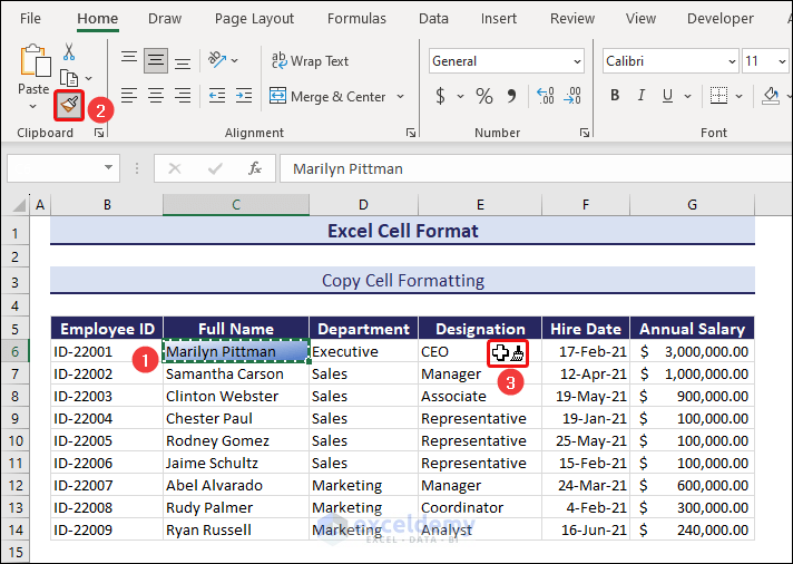
- Next, just click on cell E6. You will see the formatting of the C6 cell painted to cell E6.
Thus, you can format a cell by copying the formatting of another cell in Excel.
How to Clear Cell Format in Excel?
To clear formatting from a cell, just select the cell or range of cells and then go to the Editing group >> Clear drop-down >> Clear Formats.
Here, I cleared the formatting from C6 and E6 cells. This command returns the default formatting of a cell.
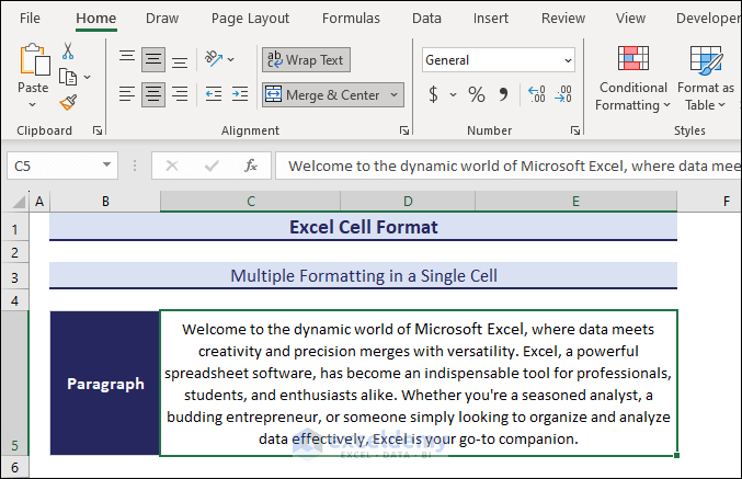
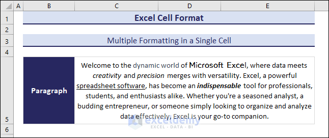
How to Perform Multiple Text Formatting in a Single Cell in Excel?
Different formatting can be done inside the same paragraph in a single cell. For instance, we can apply different font styles, sizes, and colors. You can also bold a part of a paragraph, italicize another part, underline yet another part, or change the font color for yet another part.
Let’s say you have a long paragraph inside a single cell like the following image.
Now, let’s format the font a bit.
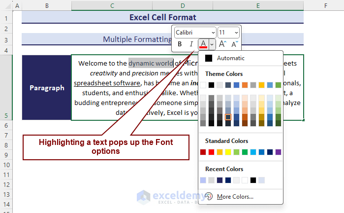
- Double-click on the cell or go to the formula bar to enable the text editing mode.
- Select a text or multiple texts.
- It will pop up the commands of the Font group automatically.
- Here, I changed the font color of the selected texts.
- In the following image, I used the keyboard shortcuts Ctrl + I, Ctrl + B, and Ctrl + U to apply Italic, Bold, and Underline commands respectively.
Thus you can perform multiple formattings in a single cell.
How to AutoFormat Cells in Excel?
Excel has some built-in formats for data tables. We can access these formats through the AutoFormat feature.
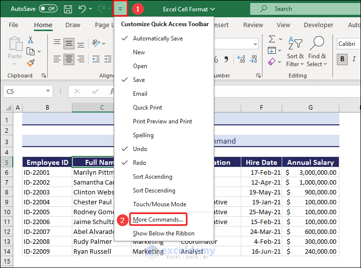
- First, we need to add this command to the Quick Access Toolbar.
- For this reason, select the Quick Access Toolbar icon ⇒ More Commands…
- After that, select All Commands from the “Choose Commands from” drop-down.
- Select AutoFormat.
- Next, click the Add ⇒ button.
- Thereafter, click OK.

Click on the image to enlarge
Now, the AutoFormat command is added to the Quick Access Toolbar. Follow the image below to understand its use.
Here, we selected the data range (B5:G14) and selected the AutoFormat command. It opens the AutoFormat dialog box and we see some formats for data tables. We chose a black-themed format here.
Download Practice Workbook
To sum up, you have learned the necessary basics about the Excel cell format after reading this article. Here, we covered the necessary tutorials on how to change cell background, increase or decrease cell size, change font style, size, color, etc. We also discussed how to apply built-in cell styles, change Cell Number Format (Default and Custom), quickly format cells using keyboard shortcuts and other features. If you have any questions or feedback regarding this article, please share them in the comment section.
Excel Cell Format: Knowledge Hub
<< Go Back to Learn Excel