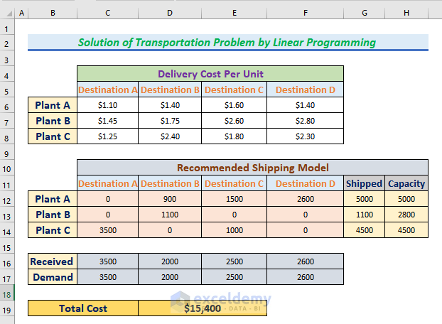
How to Solve Transportation Problem with Linear Programming

Get FREE Advanced Excel Exercises with Solutions!

The Transportation Problem is a linear programming problem that optimizes resource allocation in a transportation system. This article provides a comprehensive solution to transportation problem by linear programming in Excel, covering a procedure to find the most efficient and cost-effective way to transport goods while satisfying supply and demand constraints. Learn how to solve this complex problem with ease using Excel. Here is the overview image of the transportation problem and its solution.

Table of Contents Expand

How to Solve Transportation Problem with Linear Programming in Excel (Step-by-Step Procedures)

Solver in Excel is a powerful tool that helps optimize decision-making by finding the best solution to a problem based on constraints. It allows you to change multiple inputs and see the impact on a specific target cell. This helps find the optimal solution for complex problems in areas such as finance, operations, and marketing. Let’s have a look at the procedure for the solving method.

Step 1: Activate Solver Add-In

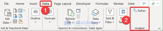
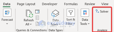
This step describes the process of activating Solver Add-Ins. Generally you will find the Solver option in the Data Tab.

If you don’t have Solver already added to your Data-Tab. Don’t even worry, the process of adding the Solver will be discussed here.

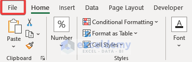
First of all, click the File.

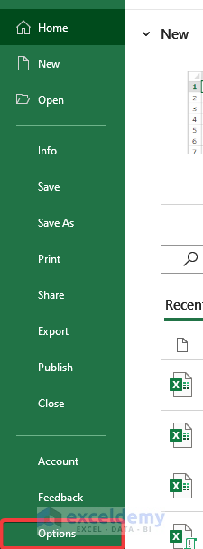
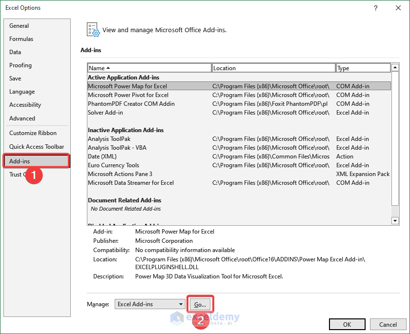
Then find the Options at the down-most corner and click it.

After then, the following tab will appear and you have to click Add-Ins. And Then click the Go as shown in the picture below.

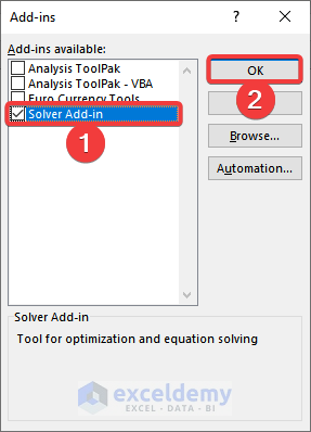
After clicking, Add-Ins available Tab will appear. From there, check the Solver Add-In. And then press OK.

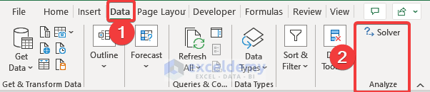
Finally, Solver will be added into the Data option.

Step 2: Create a Data Model

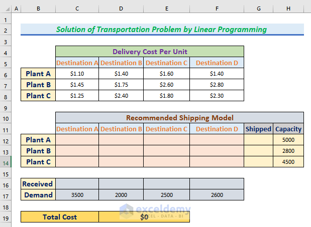
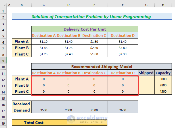
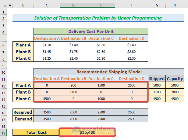
Let us assume that a manufacturing company has three plants: Plant-A, Plant-B, and Plant-C which require raw materials to transport from Destination A, Destination B, Destination C, and Destination D.

In the first table, transportation cost per unit is given.
The capacity of each plant is mentioned and the required Demand is also mentioned in the table.
Our goal is to meet the Demand at the minimum possible cost.
To calculate the cost a new Excel table named “Recommended Shipping Model” is created.

Step 3: Apply Formula to Calculate the Shipping Order

In this section, we will discuss and illustrate all the formulas used here. Make sure to follow the steps carefully.

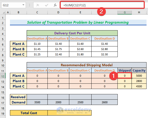
At the beginning of the work, Assign “0” ( or you can assign “1” as initial value) to all the cells from C12 to F14.

Afterwards, select the cell G12 and write down the formula as

=SUM(C12:F12)

And subsequently use Fill Handle to copy the formula to cell no G13, G14.

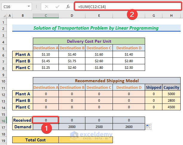
Similarly, select cell C16 and write down the formula to use the SUM Function.

=SUM(C12:C14)

To copy the formula, use Fill Handle to the cell D16 to F16.

Later, you have to select cell C19 and write down the formula as

=SUMPRODUCT(C6:F8,C12:F14)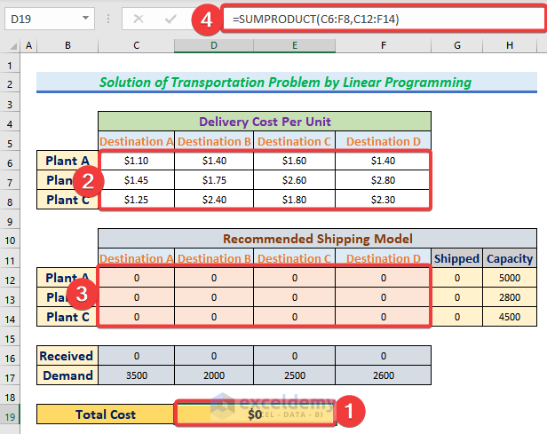

Step 4: Use of Solver Add-in

In this step, we will describe the solving procedure using the Solver Module.

Here, click the Data option and the Solver module will be available at the right corner. You have to click the Solver from the Data Option.

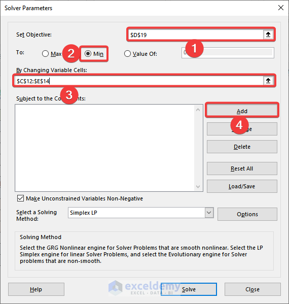
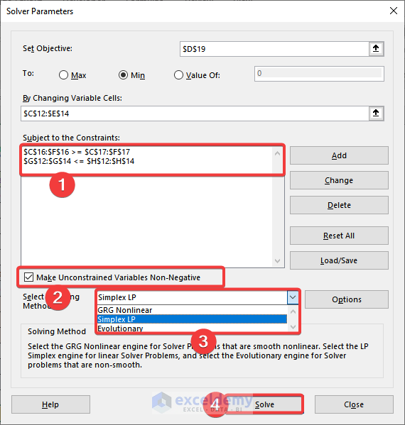
Instantly, The Solver Parameter menu will appear.
There, select D19 cell to Set Objective.
Then select Min.
In the “By Changing Variable Cell” select the cell from C12 to E14.
Immediately, click the Add icon.

Step 5: Add Subject to Constraints

Now begins the most important part of using the solver, You have to be careful about adding the Constraints.

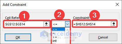
After clicking Add the new menu bar will appear. In the Add Constraint, select the cell from G12 to Then add “<=”. Eventually, in the Constraints cell select the cell from H12 to H14 to ensure the Shipped amount is always less or equal to the plant capacity.

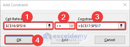
Then again click Add to insert the second Constraint. Here, Select cell C16 to F16 as Cell Reference, afterward select “=>”. Instantly after that, select the cell range from C17 to F17. Hence, press OK.

Click to “Make Unconstrained Variables Non-negative” and click on “Select Solving Technique”. From there, select Simplex LP. All the set up is done, then click the Solve.

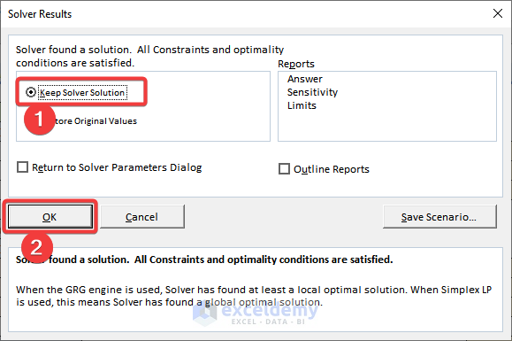
In the meantime, from the new tab named Solve Results, select Keep Solvers Solution and then press OK.

Step 6: Finding the Minimum Cost of Transportation

At last, the Solver calculates the Minimum cost of the transportation of goods while meeting the supply and demand. And the minimum cost calculated is $15400.

Download Practice Workbook

Download this practice workbook to exercise while you are reading this article.

Transportation Problem with LP.xlsx

Conclusion

In conclusion, the transportation problem is a commonly encountered optimization challenge in various industries. Linear programming provides an effective method for solving the transportation problem by maximizing profit and minimizing costs.

<< Go Back to Excel Linear Programming | Solver in Excel | Learn Excel