Data Analysis in Excel (A Comprehensive Guideline)

Get FREE Advanced Excel Exercises with Solutions!

In this article, we will learn how to analyze data in Excel. To start, we will explore different Excel functions, such as VLOOKUP, INDEX-MATCH, SUMIFS, CONCAT, and LEN functions.

Next, we will explore data analysis using Excel charts. We will learn to create various chart types, customize them, and interpret the insights they offer. We will also discuss how to apply conditional formatting effectively for data analysis purposes.

Next, we will learn how to create pivot tables, perform calculations, and generate insightful reports. Besides, we will also explore Excel’s sorting, and filtering capabilities.

We will explain the What-If Analysis feature in Excel and explore different scenarios by changing input values and observing the resulting outputs. We will also learn how to implement data validation techniques to maintain data accuracy.

Moreover, We will explore the benefits of using tables. Additionally, we will explore the built-in Analyze Data feature in Excel, which provides insights and recommendations based on your data.

For more advanced analysis needs, we will introduce the Analysis ToolPak add-in, which offers a wide range of statistical functions and tools, including descriptive analysis and ANOVA (Analysis of Variance).

By following this comprehensive guideline, you will master the skill of data analysis using Excel.

Download Practice Workbook

Download the workbook and practice.

Analyze Data in Excel.xlsx

Table of Contents Expand

How to Analyze Data in Excel

1. Use Excel Functions to Analyze Data

1.1 VLOOKUP Function

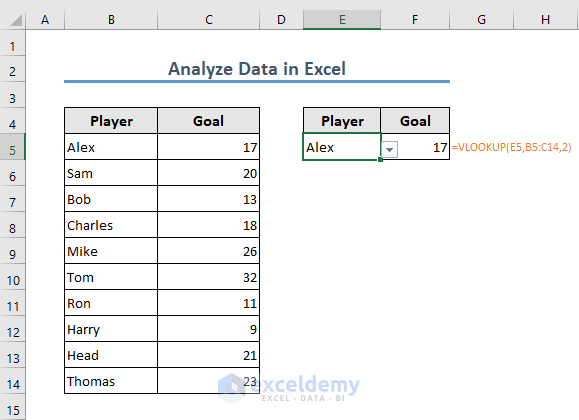
The VLOOKUP function is a frequently used function for looking up any particular data from a dataset. In the following example, I want to know how many goals an individual (for instance, Alex) has scored. The formula in cell F5 is

=VLOOKUP(E5,B5:C14,2)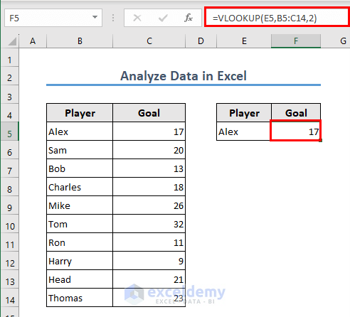

Here, Excel is looking for the value in cell E5 within the range B5:C14 and retrieving the corresponding value from the second column of that range.

1.2 INDEX-MATCH Function

You can do the same using a combination of the INDEX and MATCH functions. The formula in this case is

=INDEX(B5:C14,MATCH(E5,B5:B14,0),2)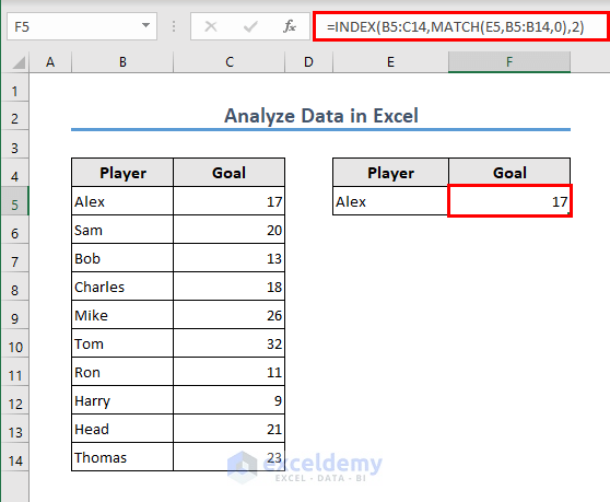

Formula Breakdown

MATCH(E5, B5:B14, 0) → The MATCH function searches for the value in cell E5 within the range B5:B14. The 0 as the third argument indicates an exact match.
Output: 1

INDEX(B5:C14, MATCH(E5, B5:B14, 0), 2) → This becomes,
↪ INDEX(B5:C14, 1, 2) → This portion retrieves the value that is in 1st row and 2nd column of the range B5:C14.
Output: 17

1.3 SUMIFS Function

The SUMIFS function is useful when you want to analyze data in Excel. It gets the sum of a range of cells with a set of conditions.

If you want to get the goals scored by the players from Group A and Group B separately, the formula you can use in cell G5 is,

=SUMIFS($D$5:$D$14,$C$5:$C$14,F5)

The formula sums the values in the range $D$5:$D$14 but only includes values where the corresponding cells in the range $C$5:$C$14 match the value in cell F5.

1.4 CONCAT Function

Even if data is in text format, you can analyze it in Excel. For example, I am going to join the first and last names of certain individuals here using the CONCAT function in Excel. The formula in cell D5 is

=CONCAT(B5," ",C5)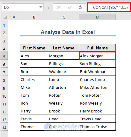

The formula joins the values in cells B5 and C5, with a space between them, resulting in a single combined text string.

1.5 LEN Function

You can count the number of characters using the LEN function. The formula in cell E5 is

=LEN(D5)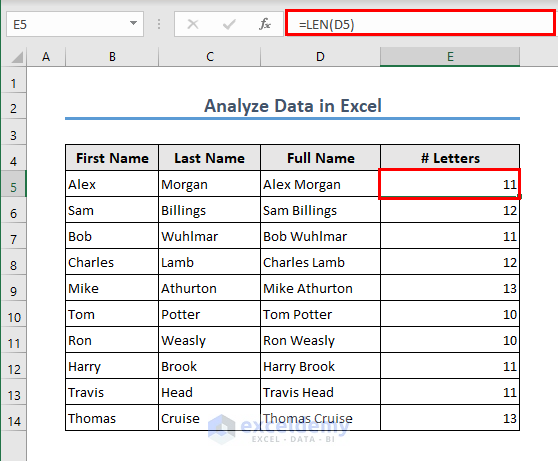

2. Data Analysis Using Excel Charts

Charts help to analyze data in Excel. Excel offers numerous types of charts so that you can illustrate your dataset in a convenient way. In our example, I will create a column chart.

Select the range F4:G6 >> go to the Insert tab >> select any column chart.

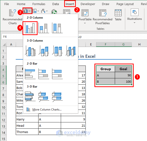
Excel will create a column chart for you.

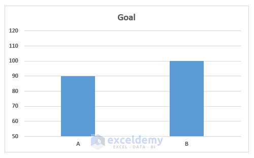
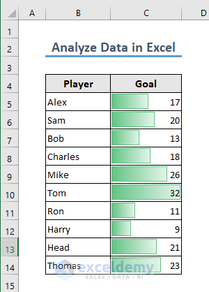
3. Apply Conditional Formatting to Analyze Data

Excel users love to apply conditional formatting to their datasets to make them visually attractive. To illustrate this, I will add data bars to the following worksheet.

Select the dataset of range C5:C14 >> go to the Home tab >> Conditional Formatting >> select a set of Data Bars.

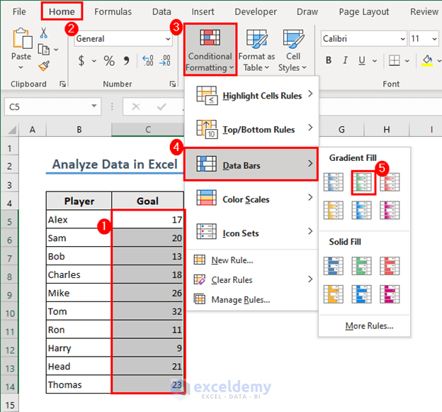
Excel will add data bars. These bars will give the dataset an excellent look.

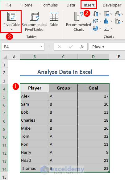
4. Pivot Table

Now, I will discuss a bit on Excel Pivot Table. Pivot tables are used for various purposes. It makes our data analysis easier in Excel. For example, I can easily calculate the number of goals scored by Group 1 and Group 2 players using the Pivot Table.

Select the dataset of range B4:B14 >> go to the Insert tab >> select PivotTable.

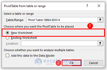
A box will appear. I have chosen a New Worksheet as the destination of my Pivot Table.

Now, drag the fields in the areas (Group in Rows and Goal in Values) shown in the image.

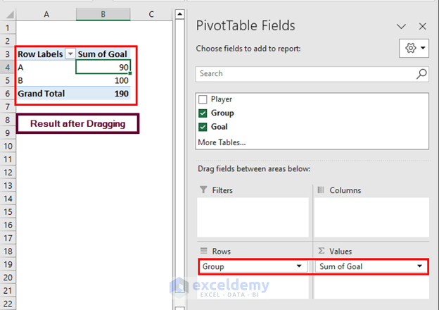
Excel calculates the sum of goals.

5. Sorting Data in Excel

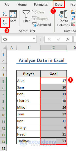
Now, let’s have a look at the Sort feature for data analysis. Suppose you want to sort the following dataset in descending order ( Largest to Smallest).

Select the range C5:C14 >> go to the Data tab >> select the Sort Z to A icon for descending order.

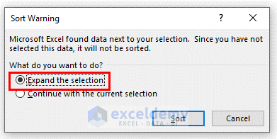
Select Expand the selection option from the warning window.

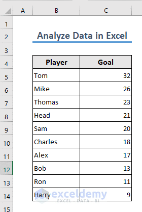
Your data will be sorted.

6. Filtering Data in Excel

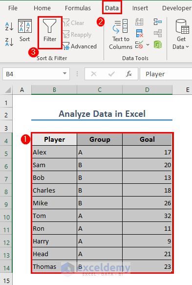
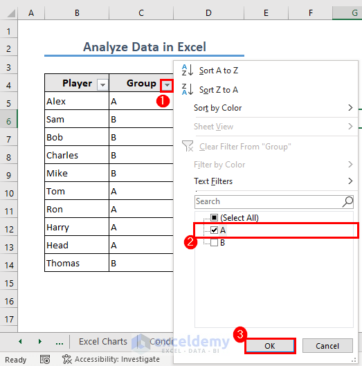
Filtering is another feature useful for data analysis. You can filter your dataset to make it tidy and get insightful information. Suppose you want to see the performance of the players of Group A.

Select range B4:D14 >> go to the Data tab >> activate Filter option.

Now filter your dataset from the drop-down icon from the column heading. I have selected Group A in the Group column.

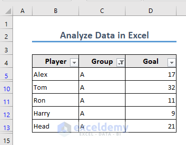
Excel will get the list of all Group A players and their performance.

7. Excel What-If Analysis Feature

What-If Analysis in Excel refers to a set of tools and techniques that allow you to explore different scenarios and observe the potential impact on the results of your formulas or models. Excel provides several features for performing what-if analysis, including:

1. Data Tables: Data Tables allow you to create a table displaying multiple results based on input values. You can perform either one-variable or two-variable data tables to see how changing inputs affect the final results.

2. Goal Seek: Goal Seek helps you determine the input value needed to achieve a specific result. You specify a target value, and Excel automatically adjusts the input value until it reaches the desired outcome.

3. Scenario Manager: Scenario Manager enables you to create and compare different sets of input values for your model. You can define multiple scenarios with varying inputs and switch between them to see the impact on the calculated results.

In this article, I will show an example of the Goal Seek feature.

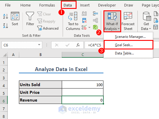
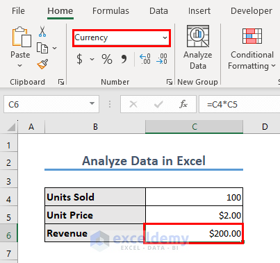
Suppose you have 100 units of a product to be sold. You want to see what will be the unit price if you want to get a revenue of $200. The formula in C6 is

=C4*C5

Now, this is very simple as we all know that the unit price will have to be $2. However, the fun with this Goal Seek feature is that you do not have to manually put the unit price. Rather, Excel will find it for you. The steps are:

Go to the Data tab >> select What-If Analysis >> select Goal Seek.

You want the revenue to be $200 and get the unit price in cell C5. So the cell to be set is C6 and the cell to be changed is C5. Put the values correctly and click OK.

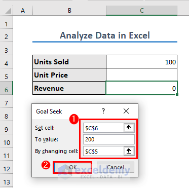
Excel will put the unit price in C5. You do not have to manually insert it. Keep the Revenue in the currency format for better clarification.

8. Data Validation

You can use the Data Validation feature to analyze data in Excel. This ensures error-free and accurate analysis in your worksheet.

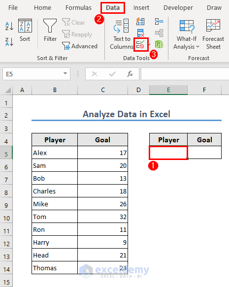
Let’s get back to our previous example (that was used to explain the VLOOKUP function). Now, we want to select a player’s name from all the available options, rather than manually typing their names.

Select cell E5 >> go to the Data tab >> select the Data Validation option.

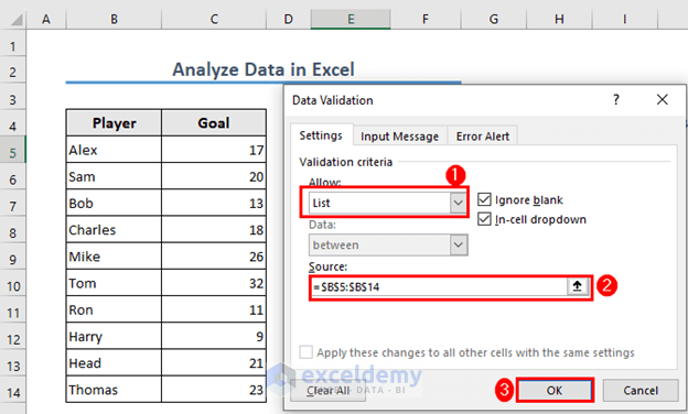
A Data Validation box will pop up.
Choose List in the Allow field >> set the sources to B5:B14 >> click OK.

Now, you can select the names from the drop-down icon.

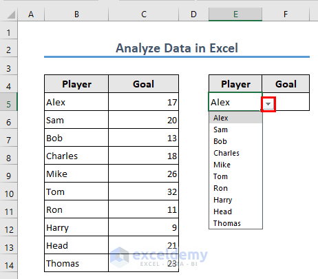
Once you select a name, you will get the number of goals the player scored.

9. Excel Table

You can use Excel tables to facilitate your data analysis in Excel. Let’s see how you can create an Excel table easily.

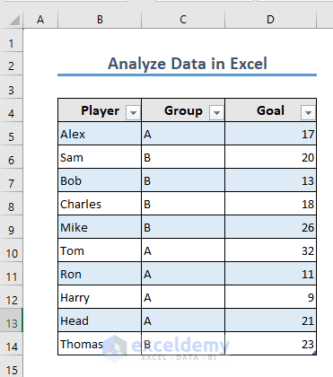
Select the dataset of range D5:D14 >> press CTRL + T >> click OK.

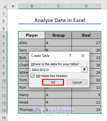
Excel will create a table.

Now, you can analyze the table in many ways. Let’s see how you can get the total goals scored by these players without using any Excel Function.

Click on any cell of the table >> Table Design tab (this tab will be seen only if you select a cell of the table first) >> Table Style Options >> check the Total Row box.

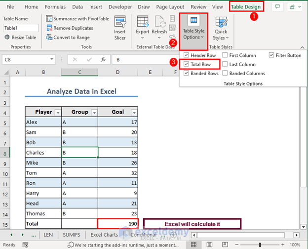
Excel shows the total goals scored.

10. Analyze Data Feature

Now, I will explain how you can use the Analyze Data feature. This feature will give you some Excel-recommended analysis techniques.

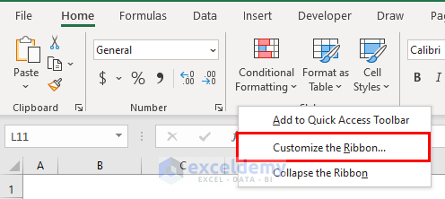
First, you have to add this feature to your ribbon. Put the cursor on the ribbon >> right-click your mouse >> select Customize the Ribbon.

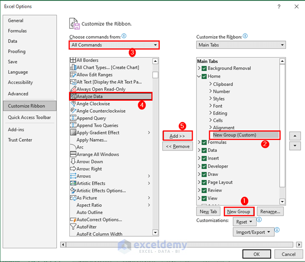
Then, add a New Group >> set its position >> select All Commands >> add Analyze Data to this newly created group >> click OK.

Now, go to the Home tab >> select Analyze Data.

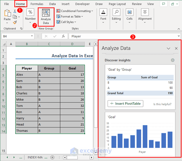
Excel is recommending several options for data analysis.

11. Use of Analysis ToolPak Add-in

You can perform tons of operations using the Analysis ToolPak add-in. First, you have to activate it.

Go to the File tab >> select Option.
Excel Options box will open.
Go to Add-ins >> select Excel Add-ins in the Manage field >> click Go.

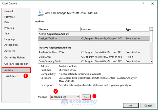
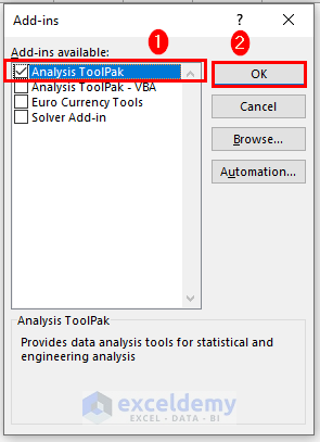
Check the box for Analysis ToolPak >> click OK.

Now, let’s do some analysis using this add-in.

Descriptive Analysis

First, we will have some descriptive analysis.

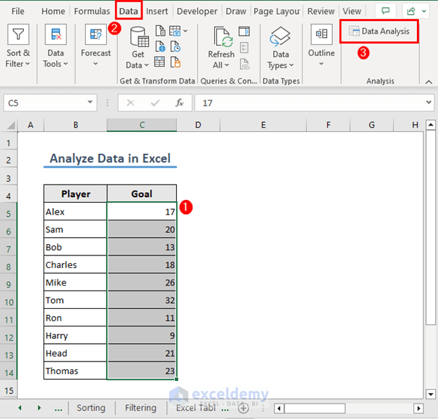
Select range C5:C14 >> go to the Data tab >> select Data Analysis (This will be available once you activate the Analysis ToolPak add-in).

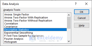
A Data Analysis box will pop up. Select Descriptive Statistics option >> click OK.

Then, set the input range and output range >> click OK.

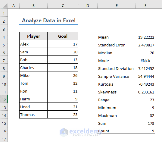
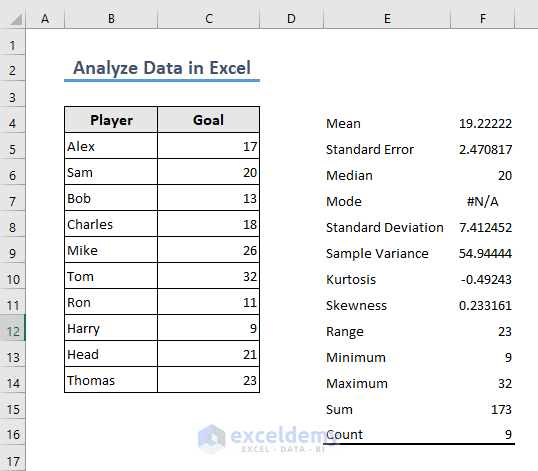
You will get the descriptive statistics of the selected input range in your Excel workbook.

ANOVA

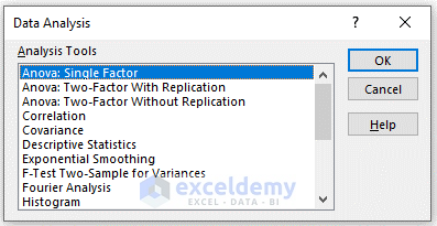
Now, we will focus on the ANOVA analysis. ANOVA stands for Analysis of Variance. It is a statistical method used to compare the means of two or more groups to determine if there are any significant differences between them.

We are looking to perform an ANOVA Single Factor analysis. So select it from the Data Analysis box and click on OK.

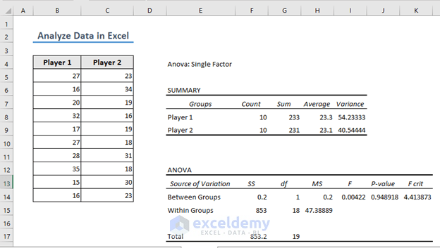
Then, set the input and output range.

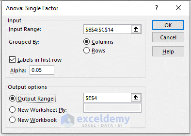
Excel will perform the operation for you.

Things to Remember

Data Validation ensures accuracy.
The INDEX-MATCH function is better than the VLOOKUP function.
You need to refresh the Pivot Table when you change your dataset.

Frequently Asked Questions

1. What are the advantages of using the Analyze Data feature in Excel over manual analysis techniques?

Ans: Advantages of using the Analyze Data feature in Excel over manual analysis techniques include saving time by automating tasks, an easy-to-use interface, lots of helpful tools and functions, the ability to customize, and working well with other Excel features.

2. What is the difference between descriptive and inferential statistics?

Ans: Descriptive statistics help describe data by summarizing it, while inferential statistics help make predictions about a larger group based on a smaller sample.

3. What are the uses of ANOVA?

Ans: ANOVA is used to compare the averages of different groups, see how categorical variables affect outcomes, analyze experiments, and understand different sources of variation in data.

Conclusion

In conclusion, this comprehensive guideline has provided you with the knowledge and skills to analyze data in Excel effectively. You have learned about useful Excel functions which help you work with and extract specific information from your data.

Excel charts have been explored to create visual representations that make it easy to understand and interpret data trends. You have also discovered how to apply conditional formatting, use pivot tables for summarizing data, and sort and filter your data.

Additionally, you have gained insight into What-If Analysis, Data Validation, Excel Table, and the Analyze Data feature. With the Analysis ToolPak add-in, you have access to advanced statistical functions like Descriptive Analysis and ANOVA.

By mastering these techniques, you can confidently analyze data in Excel and make informed decisions based on the insights you uncover.

Analyze Data in Excel: Knowledge Hub

<< Go Back to Learn Excel