In this Excel tutorial, we will learn about critical value in Excel. First, we will discuss what is critical value and the different types of critical value. Then, we will find different critical values including T, Z, F, and Chi-Square in Excel. We will also learn how to calculate the Chi-Square critical value for earlier Excel versions. We hope this article will be informative to you all.
Throughout this article, we will use Microsoft 365, but the operation applies to all versions.
To determine the significance of a hypothesis test, we use the critical value. It is calculated based on the probability distribution associated with a given set of data. Higher critical values indicate more significant results. Using critical value, one can validate hypotheses and make informed decisions about the results of a test.
Download Practice Workbook
What Is Critical Value?
The critical value determines whether the null hypothesis is rejected or not. To calculate it, we use the probability distribution associated with the data. Depending on the statistical test or distribution, we can use different functions to calculate critical value. We have a variety of critical values to choose from. To compare test statistics, we need Z critical value. The Chi-Square Critical Value is used to see if the results of the Chi-Square test are statistically significant or not. We also sometimes need T and F critical values while performing Hypothesis Tests.
How to Find T critical value in Excel?
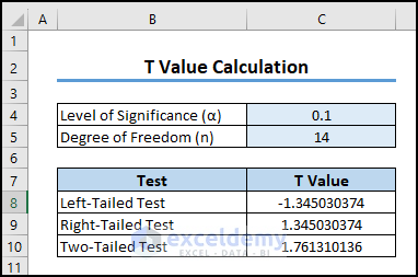
The T critical value is basically an indicator of statistical significance. The calculation process differs depending on the type of test. There are three types of tests we can perform: Left-Tailed Test, Right-Tailed Test, and Two-Tailed Test.
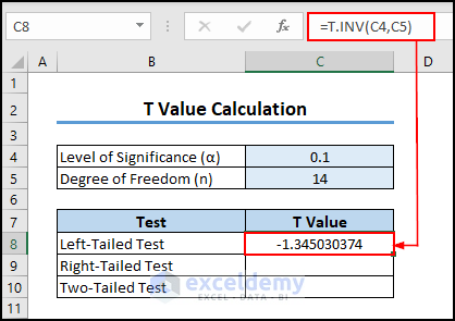
1. Use T.INV Function for Left-Tailed Test
In this method, we will use the T.INV function to calculate T critical value for a Left-Tailed Test. This function finds the two-tailed inverse value of the student’s t-distribution data.
=TINV (probability,deg_freedom)Now, follow the below steps:
- Insert the following formula in cell C8 and press Enter.
=T.INV(C4,C5)- Thus we have got T critical value for a Left-Tailed Test.
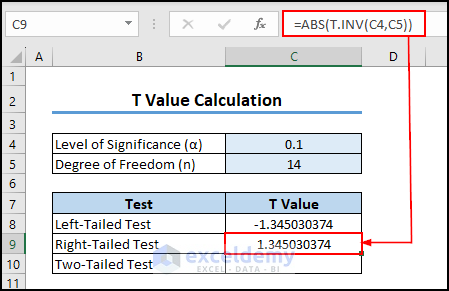
2. Combine ABS and T.INV Functions for a Right-Tailed Test
We can calculate the T critical value for a right-tailed test using the ABS function along with the T.INV function. The ABS function is used to get the absolute value of a number. We will get only a positive number in return.
=ABS(number)We can apply the ABS and T.INV functions together for a right-tailed test. To do so,
- Insert the following formula in cell C9 and press Enter.
=ABS(T.INV(C4,C5))- As a result, we have got T critical value for a Right-Tailed Test.
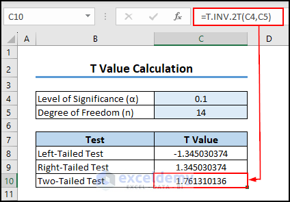
3. Apply T.INV.2T Function for Two-Tailed Test
In this part, we will apply the T.INV.2T function to calculate the T critical value for a two-tailed test. This function returns the two-tailed inverse value of the student’s t-distribution data.
=T.INV.2T (probability,deg_freedom)Now, go through the below steps:
- Insert the following formula in cell C10 and press Enter.
=T.INV.2T(C4,C5)- Thus we have got the result.
How to Find Z Critical Value in Excel?
Z critical value is a statistical term used to determine a hypothesis’s statistical significance. It is important to consider the population parameters in this case. There are three types of Z critical value tests: Left-Tailed Test, Right-Tailed Test, and Two-Tailed Test.
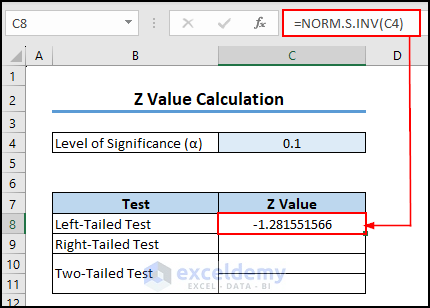
1. Calculate Z Critical Value for Left-Tailed Test
We will calculate the Z critical value for a Left-tailed test using the NORM.S.INV function. The NORMINV function returns the inverse of the standard normal cumulative distribution (has a mean of zero and a standard deviation of one).
=NORM.S.INV(probability)Now, follow the below steps:
- Insert the following formula in cell C8 and press Enter.
=NORM.S.INV(C4)- In this way, we got the Z critical value for a Left-tailed test.
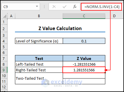
2. Find Z Critical Value for Right-Tailed Test
In this section, we will explain how to calculate Z critical value for a right-tailed test using the NORM.S.INV function. Here are the steps:
- Insert the following formula in cell C9 and press Enter.
=NORM.S.INV(1-C4)- As a result, we will get the Z critical value.
3. Determine Z Critical Value for Two-Tailed Test
We can compute the Z critical value for two-tailed tests. There are two values corresponding to a two-tailed test. We will use the same NORM.S.INV function to determine the Z critical value. To do so,
- Insert the following formula in cell C10 and press Enter to get the first value.
=NORM.S.INV(C4/2)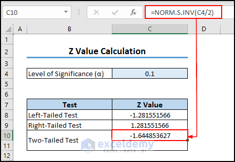
- Similarly, for the second value, insert the following formula in cell C11 and press Enter.
=NORM.S.INV(1-C4/2)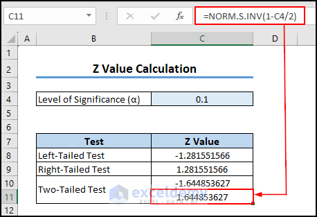
Read More: How to Find Z Critical Value in Excel
How to Find F Critical Value in Excel?
The F critical value is a number that is used to compare your F-value. You will be able to find the F critical value in Excel when you know the probability, the degree of freedom of the Numerator, and the degree of freedom of the Denominator. To calculate F critical value, follow the below steps:
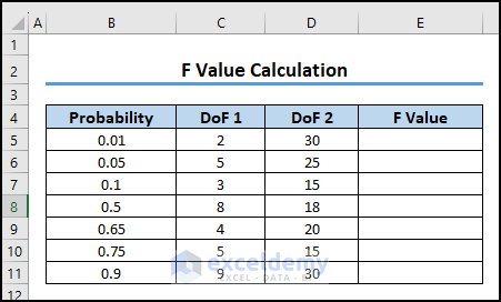
Step 1: Create Dataset
In this section, we will create a dataset to find F critical value in Excel. As we use the F.INV.RT function to find the F critical value, the function has three arguments. So we need a dataset that has 3 columns, and we also need another extra column to find the F critical value. We will create a column named “ F value”.
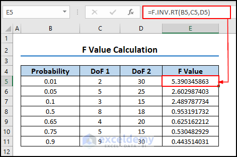
Step 2: Use F.INT.RT Function
Now, we will use the F.INT.RT function to calculate the F critical value in Excel. The F.INT.RT function returns the inverse of the (right-tailed) F probability distribution. If p = F.DIST.RT(x,…), then F.INV.RT(p,…) = x.
=F.INV.RT(probability,deg_freedom1,deg_freedom2)To calculate the F critical value, follow the steps below:
- Insert the following formula in cell E5 and press Enter.
- After that, AutoFill the formula to the rest of the cell in column E.
=F.INV.RT(B5,C5,D5)- As a result, we will get all the F critical values in Excel.
Read More: How to Find F Critical Value in Excel
How to Find Chi-Square Critical Value in Excel?
We use the Chi-Square critical value to check whether the results of the Chi-Square test are statistically significant or not. The test findings are statistically significant if the test statistic is larger than the Chi-Square critical value. Here, we will discuss two ways of calculating the Chi-Square critical value.
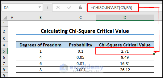
1. Use CHISQ.INV.IRT Function to Find Chi-Square Critical Value
We can use the CHISQ.INV.IRT function to find Chi-Square critical value in Excel. The CHISQ.INV.IRT function returns the inverse of the right-tailed probability of the chi-squared distribution.
=CHISQ.INV.RT(probability,deg_freedom)Here are the required steps you need to follow:
- Insert the following formula in cell D5 and press Enter.
- Then drag down the Fill Handle to apply the formula to the rest of the cell in column D.
=CHISQ.INV.RT(C5,B5)- Thus, we got our desired Chi-Square critical values.
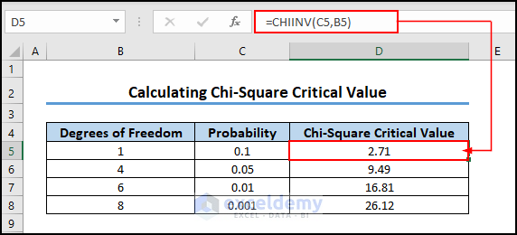
2. Find Chi-Square Critical Value for Earlier Excel Versions
If we use Excel 2007 and earlier versions of Excel, then the CHISQ.INV.RT function is not available there. In the earlier versions, we have to use the CHIINV function instead of the CHISQ.INV.RT function. The CHIINV function returns the inverse of the right-tailed probability of the chi-squared distribution.
=CHIINV(probability,deg_freedom)Now, go through the steps below to find Chi-Square critical value:
- Insert the following formula in cell D5 and press Enter.
- Then AutoFill the CHIINV function to the rest of the cell in column D.
=CHIINV(C5,B5)- As a result, we got our desired Chi-Square critical values like the below image.
Frequently Asked Questions
1. What should I do if my desired significance level is not a standard value like 0.05 or 0.01 in Excel?
Answer: You can still find critical values if your significance level is not a standard value by using Excel’s interpolation functions, such as LINEST or FORECAST, or by interpolating between critical value tables.
2. What is the critical value for the 95 confidence interval in Excel?
Answer: A 95% or 0.95 confidence interval corresponds to alpha (α) = 1 – 0.95 = 0.05.
3. Are critical values the same for every statistical test in Excel?
Answer: Excel’s critical values are not the same for every statistical test. Depending on the type of test, the distribution of the data, the sample size, and the significance level, critical values can vary. There are different critical value calculations for different tests.
What Are the Key Takeaways from This Article?
- Here, we have discussed all necessary topics about critical value in Excel.
- Explained what is the critical value.
- Discussed how to find different critical values including T, Z, F, and Chi-Square in Excel.
- Showed how to find Chi-Square critical values for earlier Excel versions.
- Provide solutions to frequently asked questions by readers.
Conclusion
Throughout the article, we’ve covered everything you need to know about critical value in Excel. We have discussed how to find different critical values including T, Z, F, and Chi-Square in Excel. We hope you found this article informative and useful. Feel free to leave any questions, comments, or recommendations in the comments section.
Critical Value In Excel: Knowledge Hub
- How to Find Critical Value in Excel
- Find Chi-Square Critical Value in Excel
- Critical Value of r in Excel
- How to Find T Critical Value in Excel
<< Go Back to Excel for Statistics | Learn Excel

