This article will demonstrate various methods to check, count, remove, and filter duplicates in Excel.
You will learn how to
– Highlight duplicates
– Count the number of duplicates
– Remove duplicates
– Find duplicate rows and
– Filter duplicates.
Identifying duplicates and filtering or removing them is significant in reducing file size and also helps in data processing by removing duplicates allowing easier data management.
Download Practice Workbook
What are the Different Methods to Check Duplicates in Excel?
To check duplicates in Excel, we will use 4 different methods including Conditional Formatting, the COUNTIF function, the VLOOKUP function, and lastly, a combined formula of the IF function, the SUM function, and the EXACT function. These methods will help us find out the duplicates and better visualize them. The proper steps along with appropriate examples are described below.
1. Using Conditional Formatting
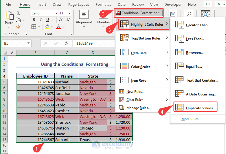
To check duplicates, we’ll use Conditional Formatting in this method. This will help us better visualize them throughout the dataset. The steps are below.
📌 Steps:
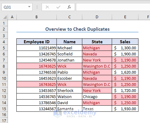
- Firstly, select the entire dataset without the headers (cell B5:E15).
- Then, go to the Home tab => Conditional Formatting => Highlight Cells Rules => Duplicate Values.
- In the dialog box that appears, click OK. This will highlight the duplicate cells like in the image below.
Click on the image for better quality
2. Using the COUNTIF Function
To check duplicates, we’ll use the COUNTIF function in this method. This will give us the number of duplicates in the entire worksheet. This is efficient in determining the number of duplicates that helps in data processing and transformation processes.
For this method, apply the following formula to count the number of duplicates.
=COUNTIF($D$5:$D$15,D5)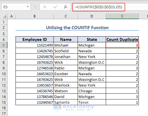
3. Case-sensitive Duplicates in Excel
To check case-sensitive duplicates in Excel, we will use a formula containing different functions. In our example, we inserted New York and new York as State and the formula will count them as separate.
For testing the case sensitivity, insert the following formula in a cell to count case-sensitive duplicates.
=IF(SUM((--EXACT(D5:D15,D5)))<=1,"Not Duplicate","Duplicate")
💡Formula Breakdown
- The EXACT function is used to compare each cell in the range (D5:D15) with the value in cell D5. It returns an array of TRUE or FALSE values, where TRUE indicates an exact match and FALSE indicates a mismatch.
- The double negation (—) is applied to the array of TRUE or FALSE values using the unary operator. This converts TRUE to 1 and FALSE to 0.
- The SUM function is used to add up the resulting array of 1s and 0s. The sum represents the number of exact matches found in the range.
- The IF function is used to evaluate the sum. If the sum is less than or equal to 1 (meaning there is either no duplicate or only one occurrence), it returns “Not Duplicate“. Otherwise, it returns “Duplicate“.
4. Using the VLOOKUP Function
To check duplicates in Excel, we can also use the VLOOKUP function. In a separate column, it shows the duplicate status. The formula for the column cells is below.
=IFERROR(VLOOKUP(D5, $C$5:$C$15, 1, FALSE), "No Duplicate")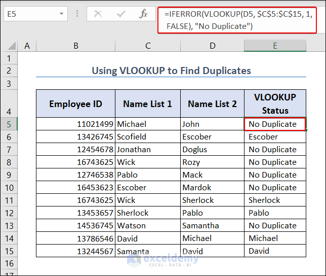
💡Formula Breakdown
- The VLOOKUP function searches for the value in cell D5 (the lookup value) within the range $C$5:$C$15 (the lookup range). The value to be returned is the first column in the lookup range (column 1), and the last argument, FALSE, specifies an exact match.
- If a match is found, VLOOKUP returns the matched value from column 1 of the lookup range.
- If no match is found, VLOOKUP returns an error.
- The IFERROR function checks if the VLOOKUP function returns an error. If an error occurs (indicating no match), it returns “No Duplicate“. Otherwise, it returns the matched value.
What are the Different Methods to Remove Duplicates in Excel Based on Columns?
To remove duplicates in Excel, we will use these 2 methods including the use of the Ribbon and Conditional Formatting. Removing duplicates helps to reduce file size and makes the data transformation process easy. Description of these methods with appropriate examples and steps are below.
1. Using the ‘Remove Duplicates’ Feature
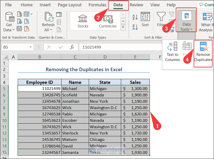
To remove duplicates in Excel, we will use the Data tab in the Ribbon. This is the fastest way to get the job done. Follow the steps below.
📌 Steps:
- Primarily, select the dataset and open the Data tab > Remove Duplicates.
- Then, in the Remove Duplicates dialog box, click on My Data Has Headers => click on OK.
Click on the image for better quality
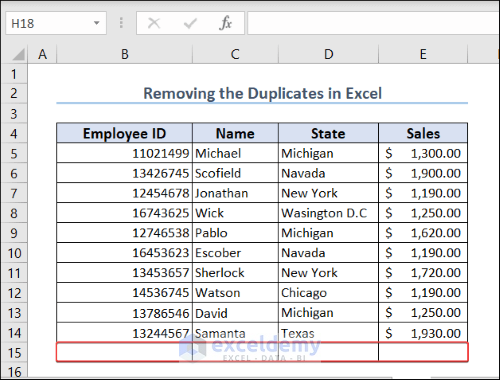
- Finally, we will see the duplicates removed.
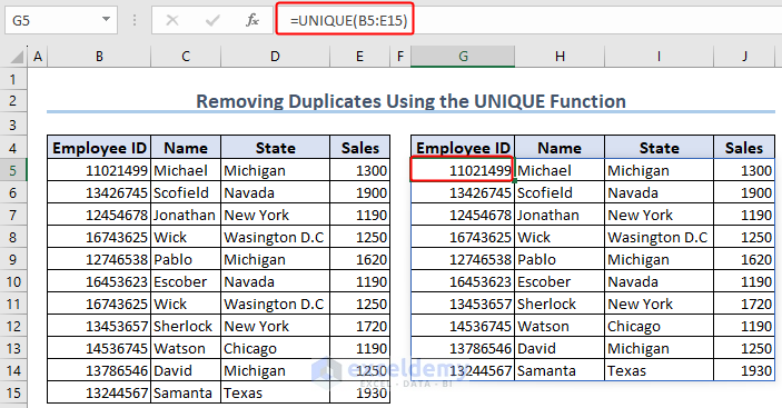
2. Using Excel ‘UNIQUE’ Function
For removing duplicates in Excel, we can also use the UNIQUE function. It will show only the unique values. However, this formula is available only in Excel for Microsoft 365 and Excel 2021 versions.
An overview of the UNIQUE function is below.
For applying the UNIQUE function, select any blank cell and input the formula in the formula box.
This will immediately give the unique data combining those columns. The output along with the formula.
3. Using Conditional Formatting
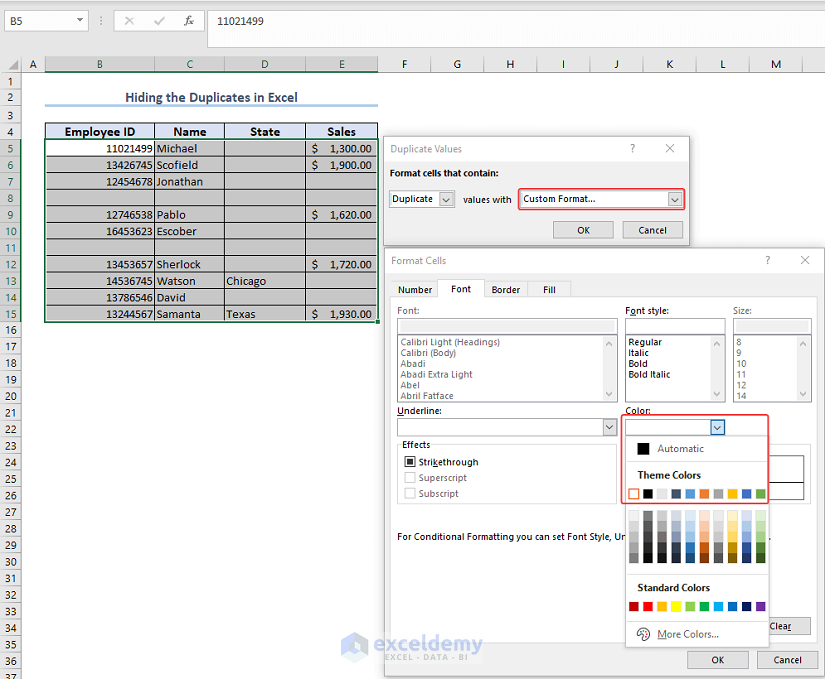
This method does not actually Remove duplicates, rather it Hides them using different formatting. This type of action is needed when we need to visualize the unique data only. The steps are below.
📌 Steps:
- First, open Conditional Formatting > Duplicates.
- Then, choose Custom Format from the dropdown menu on the right in the Format Cells dialog box.
- Finally, choose the same color as the workbook background for duplicates in the Format Cells dialog box. This will hide them visually.
Click on the image for better quality
How to Check Duplicate Rows in Excel?
To check duplicate rows in Excel, we will need a separate column that will say if the row is duplicate beside it. This also includes using a formula. The advantage of the process is that we can easily filter later on based on the status of that column.
To do so, apply the following formula.
=IF(COUNTIFS($B$5:$B$15,$B5,$C$5:$C$15,$C5,$D$5:$D$15,$D5)>1,"Duplicate row","No Duplicate")
💡Formula Breakdown
- The COUNTIFS function is used to count the number of rows that meet multiple criteria. In this case, it counts the number of rows where:
- The value in column B matches the value in cell B5.
- The value in column C matches the value in cell C5.
- The value in column D matches the value in cell D5.
- If the count is greater than 1, it indicates that there are multiple rows that satisfy all the specified criteria.
- The IF function checks if the count is greater than 1. If so, it returns “Duplicate row“. Otherwise, it returns “No Duplicate“.
How to Filter Duplicates by Their Occurrences?
To filter duplicates by their number of occurrences, we can first use the COUNTIF formula to count the number of occurrences as we mentioned in the previous method. Then we will sort them based on those numbers. Follow the steps below.
📌 Steps:
- Firstly, select the dataset and go to the Home tab => Editing => Sort & Filter.

Click on the image for better quality
- Later on, click on the filter in the Duplicate Status column.
- Then, select Number Filters => Greater Than.
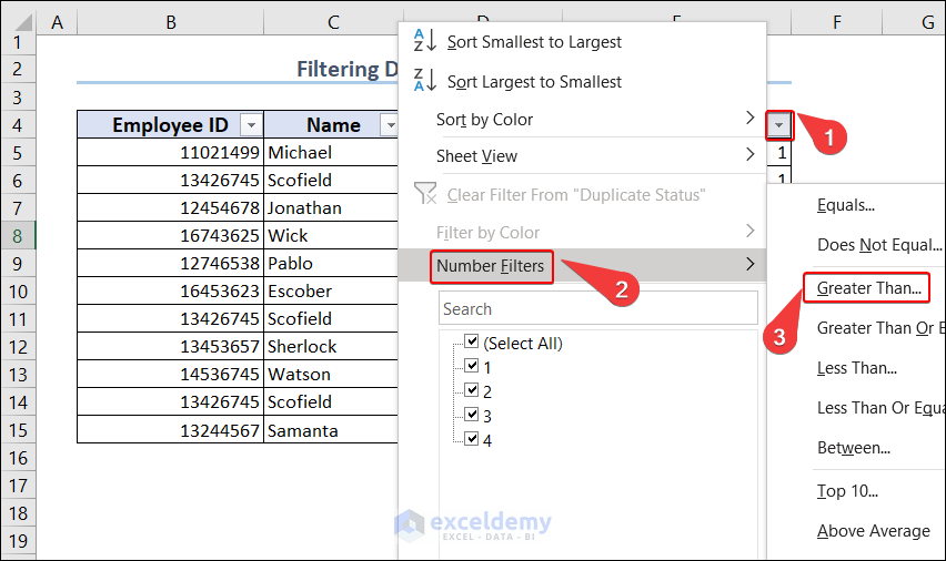
Click on the image for better quality
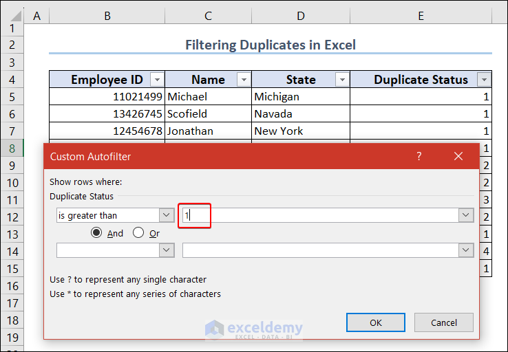
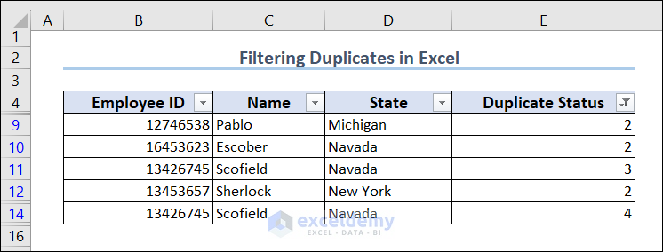
- Lastly, select 1 as the Is greater than Press OK.
- Finally, you will get the duplicates removed.
Things to Remember
- Sometimes, we used absolute cell reference with the “$” sign to keep the formula intact while copying.
- To filter duplicates by their occurrences, we need a separate column containing the number of occurrences using the COUNTIF function shown in the previous method.
- Don’t forget to use the Fill Handle to copy the formula for all the cells needed.
- Conditional Formatting does not affect the values. it changes the appearance, so the data is still accessible.
Frequently Asked Questions
Q1. What are duplicates in Excel?
Answer: Duplicates in Excel refer to the same values or entries that appear more than once in a column or range of cells within a worksheet.
Q2. Can I specify the criteria for identifying duplicates in Excel?
Answer: Yes, you can specify criteria to identify duplicates in Excel. In the Remove Duplicates dialog box, you can choose which columns to include in the duplicate comparison. By selecting specific columns, you can establish criteria for determining duplicates based on the values in those columns.
Q3. Is there a way to find duplicates across multiple worksheets?
Answer: Yes, you can find duplicates across multiple worksheets by using Excel’s Power Query (Get & Transform Data) feature. First, you will need to combine and analyze data from multiple worksheets. Then you will be able to apply the Remove Duplicates feature. This will remove duplicates across different sheets.
Conclusion
Throughout this tutorial, you have learned different methods related to finding out, removing, and filtering duplicates in Excel. Different methods and multiple applications have been shown here for better understanding. Here we used Conditional formatting, the COUNTIF function, the IF function, the VLOOKUP function, their combination, etc. This will help you to check duplicates, find out the number of duplicates, filter them, and remove them as well.
Check out the Knowledge Hub section below for similar articles related to Duplicates in Excel. If you’re still having trouble with any of these examples or methods, let us know in the comments. Our team is ready to answer all of your questions. For any Excel-related problems, you can visit our website, Exceldemy, for solutions.
Duplicates in Excel: Knowledge Hub
- Count Duplicates in Excel
- Merge Duplicates in Excel
- Find Duplicates in Excel
- Highlight Duplicates in Excel
<< Go Back to Learn Excel

