The TRUNC function in Excel truncates a number to a specified number of digits. It is under the category of Excel Math and Trigonometry function. The function is mainly used for removing the decimal parts from a number.
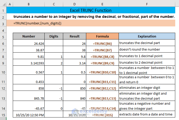
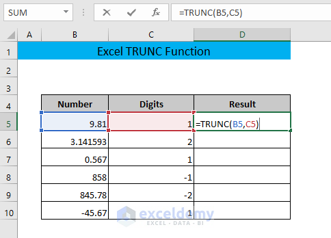
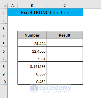
From the above image, we can get a general overview of the TRUNC function. Throughout the article, we will see the details of this function.
Introduction to the TRUNC Function
❑ Objective
Excel TRUNC function truncates a number to an integer by removing the decimal, or fractional, part of the number.
❑ Syntax
TRUNC(number,[num_digits])
❑ Argument Explanation
| Argument | Required/Optional | Explanation |
|---|---|---|
| number | Required | A number which will be truncated |
| num_digits | Optional | The number of decimal places to return in the truncated number. If this argument is omitted, there will be no decimal part in the returned number. |
❑ Output
The TRUNC function returns a truncated numeric value.
❑ Version
This function is available from Excel 2000. So any version since Excel 2000 has this function.
How to Use TRUNC Function in Excel: 4 Examples
Now, we will see different examples where various applications of the TRUNC function are shown.
1. Remove Decimal Parts of a Number
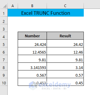
We can remove decimal parts of a number by using the TRUNC function. Suppose we have a dataset where we have some numbers with decimal points. Now, we will apply the TRUNC function to remove the decimal parts of the numbers.
➤ Type the following formula in cell C5,
=TRUNC(B5)
The formula will truncate the number of the cell B5 in such a way that there will be no decimal parts in the returned number.
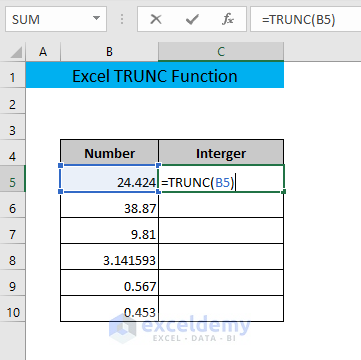
➤ After that, press ENTER.
As a result you will get the integer part of the number of cell B5 in cell C5.

➤ Now drag the cell C5 to the end of your dataset to apply the same formula for all of the numbers.

If you observe you can see that the TRUNC function returns zero for any number between 0 to 1.
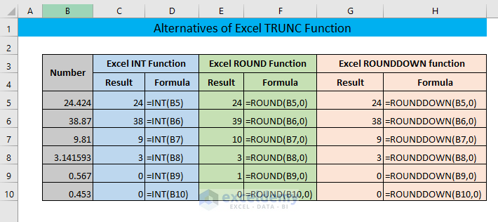
We can use other functions such as Excel INT function, Excel ROUND function, or Excel ROUNDDOWN function instead of the TRUNC function to remove decimal parts of a number. The application of these functions for this example is shown in the image below.
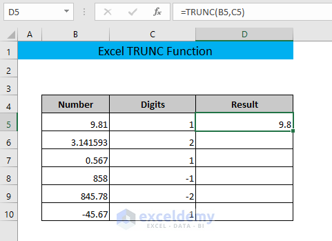
2. Shorten a Number to a Specific Digit with TRUNC Function
Excel TRUNC function can shorten a number to a specific digit. Let’s say, we have some numbers in our dataset in column B and the number of digits we want after the decimal point are given in column C. Now, we will use the TRUNC function to shorten these numbers to specified digits.
➤ First, type the formula in cell D5,
=TRUNC(B5,C5)The formula will shorten the number of cell B5 to the specified digit of cell C5 and will return the shortened number in cell D5.
➤ Press ENTER.
And we will get the shortened number in cell D5.
➤ At last, drag the cell D5 to the end of your dataset.
As a result, we will get all the numbers shortened to the specific digits we have mentioned in column C.
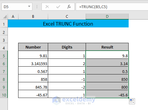
If you carefully observe cells C8 and C9 have negative numbers as the digits. The formula eliminates digits from the integer part of the number and returns 0 at that place when the specified digit is negative.
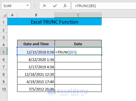
3. TRUNC Function to Remove Time from Date and Time Cells
TRUNC function can also be used to remove time from date and time cells. Suppose at this time we have some dates and times in our dataset. We want to remove the time part and extract only the date part from these dates and times.
➤ First type the following formula in cell C5,
=TRUNC(B5)The formula will truncate the time portion from the date and time of cell B5.
➤ After that, press ENTER
As a result, you will see the time portion is showing 0:00 in cell C5.
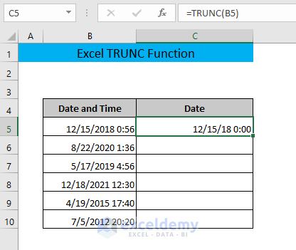
➤ Drag the cell C5 to the end of your dataset to apply the same formula for all other dates and times.
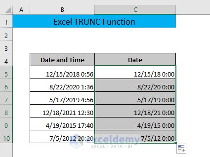
We can remove the 0:00 from these cells. To do that,
➤ Go to Home > Number and select Short Date.
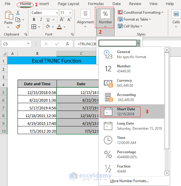
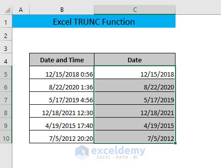
As a result, you will see 0:00 is removed from the cells. Now, we have only the dates.
Read More: How to Truncate Date in Excel
4. TRUNC Function in VBA
TRUNC is not a part of the application.worksheetfunction. As a result, it can’t be utilized in Excel VBA. But, we can apply the FORMAT function to achieve the same result. Suppose we have the following dataset where we want to convert the number with two decimal points.
To do that first,
➤ Press ALT+F11 to open the VBA window and press CTRL+G to open the Immediate box in the VBA window.
After that,
➤ Insert the following code in the Immediate box line by line and press ENTER after every line.
Range("C5") = Format(Range("B5"), "##.##")
Range("C6") = Format(Range("B6"), "##.##")
Range("C7") = Format(Range("B7"), "##.##")
Range("C8") = Format(Range("B8"), "##.##")
Range("C9") = Format(Range("B9"), "##.##")
Range("C10") = Format(Range("B10"), "##.##")
The code will return the numbers of column C with two decimal points in column D.

➤ Close the VBA window.
Now, you will see the numbers with two decimal points in column C.
Read More: How to Use Truncate in Excel VBA
💡 Things to Remember When Using TRUNC Function
📌 The TRUNC function will give #VALUE! error, if you give input in text format.
📌 The INT function and the ROUNDDOWN function give the same result as the TRUNC function. However the TRUNC function is easier to use because it requires fewer arguments.
📂 Download Practice Workbook
Conclusion
I hope now you know how the Excel TRUNC function works and how to apply the function in different conditions. If you have any confusion, please feel free to leave a comment.
TRUNC Function in Excel: Knowledge Hub
<< Go Back to Excel Functions | Learn Excel

