In this article, we will learn about the ADDRESS function in Excel. We will also explore how to return cell value by address, cell address instead of value, and cell address of match.
The ADDRESS function in MS Excel is under the Lookup and Reference functions category. We use the ADDRESS function to get the address of a cell in an Excel worksheet in text form given specified the corresponding row and column numbers. The ADDRESS function can return the cell address in Absolute, Mixed, or Relative reference format with corresponding input. The address can also be used as the cell reference inside another formula.
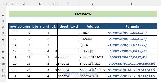
The following picture is an overview of the uses of the ADDRESS function.
Introduction to the ADDRESS Function in Excel

Function Objective:
The ADDRESS function is used to create a cell reference as text, given specified row and column numbers.
Available in:
Excel 2007 to Excel 2021 versions & Excel 365.
Syntax:
=ADDRESS(row_num, column_num, [abs_num], [a1], [sheet_text])
Arguments:
| Argument | Required/Optional | Explanation |
|---|---|---|
| row_num | Required | This refers to the row number in the cell reference. |
| column_num | Required | This refers to the column number in the cell reference. |
| abs_num | Optional | This specifies the type of cell reference to return.
|
| a1 |
Optional | This is a logical value that specifies the A1 or R1C1 reference style.
|
| sheet_text |
Optional | This indicates the sheet address of the reference. If this argument is omitted, it refers to the cell being on the current sheet. Example: ‘Sheet1’R5C[2]. |
Use of Required and Optional Arguments:
| Formula | Description | Output |
|---|---|---|
| =ADDRESS(1,1,1,0,”[Book1]Sheet1″) | Absolute reference to another worksheet in another workbook in R1C1 style | ‘[Book1]Sheet1’!R1C1 |
| =ADDRESS(1,1,2,0,”[Book1]Sheet1″) | Absolute row; relative column to another worksheet in another workbook in R1C1 style | ‘[Book1]Sheet1’!R1C[1] |
| =ADDRESS(1,1,4,0,”[Book1]Sheet1″) | Relative reference to another worksheet in another workbook in R1C1 style | ‘Book1]Sheet1’!R[1]C[1] |
| =ADDRESS(1,1,1,1,”[Book1]Sheet1″) | Absolute reference to another worksheet in another workbook in A1 style | ‘[Book1]Sheet1’!$A$1 |
| =ADDRESS(1,1,2,1,”[Book1]Sheet1″) | Absolute row; relative column to another worksheet in another workbook in A1 style | ‘[Book1]Sheet1’!A$1 |
| =ADDRESS(1,1,4,1,”[Book1]Sheet1″) | Relative reference to another worksheet in another workbook in A1 style | ‘[Book1]Sheet1’!A1 |
In the upcoming sections, we will see several examples of how we can use this Excel function for different purposes.
How to Use ADDRESS Function in Excel: 7 Suitable Examples
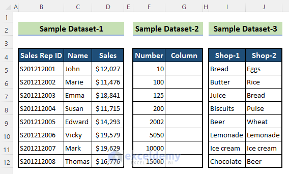
To explore the usage of the ADDRESS function, keep going through the following examples. Before we start, let’s see the following datasets that we are going to use in our demonstration.
Example 1: Basic Use of ADDRESS Function in Excel
In the first example, we will learn the basic use of the ADDRESS function.
Simple Cell Address When Only the Row and Column Numbers are Given:
In such cases, the ADDRESS function returns the cell address in A1 reference style (column letter together with the row number), in Absolute Cell Reference by default, and considers the cell in the current worksheet.
📌 Steps
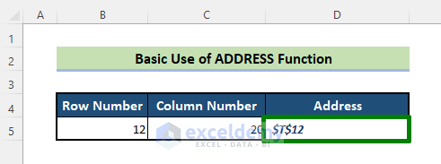
- First of all, specify the row and column number in Cell B5 and C5 and enter the following formula in Cell D5 to get the corresponding cell address:
=ADDRESS(B5,C5)

- After pressing the ENTER key, the function returns the cell address in the format as stated above. The address is $T$12.
Cell Address with Reference Type, Style, and Sheet Location Given:
Let’s see the same example.
Full Formula:
=ADDRESS(B5,C5,4,0,B8)📌 Steps
- Double-click on Cell D5 > Type
ADDRESS(B5,C5> Put a comma and then a space after C5.
See what happens. 👇

So, if you type 1, you will get the cell address in the absolute reference, if 2,3 or 4 is typed, then you will get absolute row/relative column, relative row/absolute column, and relative reference respectively.
- Type 4 after the comma, type another comma and see Excel shows the following options. 👇

If you type 0 (zero), you will get the cell address in R1C1 style. If you type 1, you will get the cell address in A1 style.
- Type 0 after the comma. Type another comma, and type your sheet name in double quotes like “Example 1”. If you have a list of sheet names, click on the cell that contains the specific sheet name.

- Hit ENTER.
The following picture shows the cell address. It’s ‘Example 1’!R[12]C[20].

The ADDRESS function returns the cell address in two reference styles. A1 and R1C1.
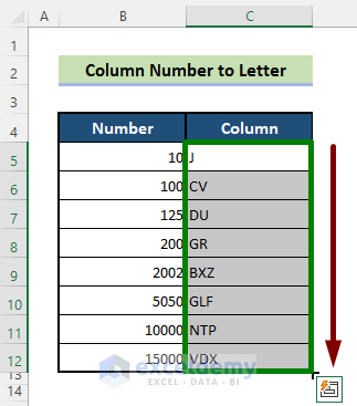
Example 2: Convert Column Number to Letter with Excel ADDRESS Function
We can convert Column Number to Column Letter, and Column Letter to Number using the SUBSTITUTE function with the ADDRESS function. To do that, follow the steps below.
📌 Steps
- Enter the formula below in Cell C5.
=SUBSTITUTE(ADDRESS(1,B5,4),"1","")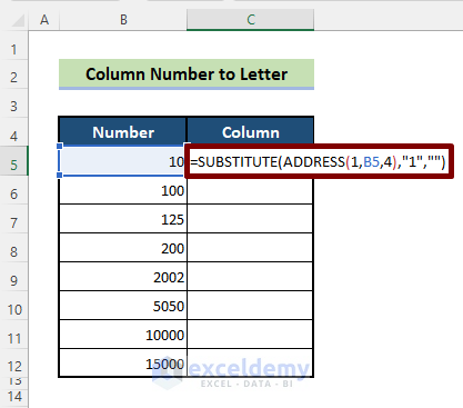
- Press ENTER and drag the Fill handle icon all the way.
The following picture shows the Column Letters generated from certain Column Numbers.
🔎 Explanation
- ADDRESS(1,B5,4)
The ADDRESS function returns the address in relative reference style.
Output: “J1”.
- SUBSTITUTE(ADDRESS(1,B5,4),”1″,””)
The SUBSTITUTE function substitutes 1 with an empty string “”.
Output: “J”.
In the SUBSTITUTE function, we can keep substituting “1” with “” as 1 is hardcoded in the function.
Example 3: Addresses of the First and the Last Cells in a Range
The Excel ADDRESS function can return the addresses of the first and the last cells in a range of data when combined with other Excel functions like MIN, ROW, MAX, and COLUMN. You wonder, how is that? Let’s see then.
📌 Steps
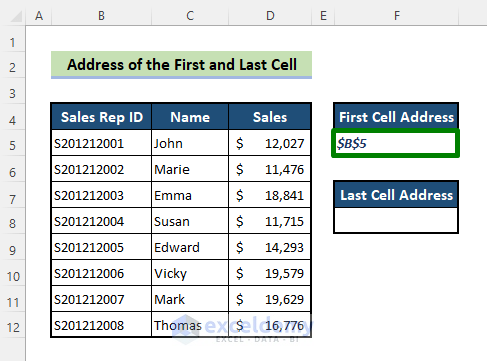
- To find the First Cell’s address, enter the following formula in Cell F5:
=ADDRESS(MIN(ROW(B5:D12)),MIN(COLUMN(B5:D12)))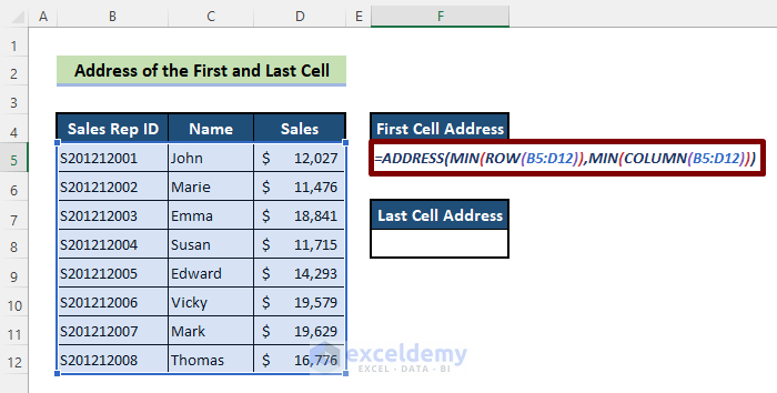
- Press ENTER.
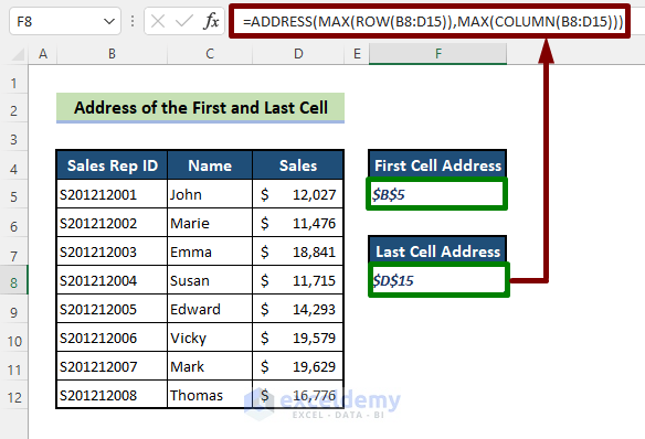
- Enter the following formula for the last cell’s address:
=ADDRESS(MAX(ROW(B8:D15)),MAX(COLUMN(B8:D15)))- Press ENTER.
Look at the following screenshot.
🔎 How Does the Formula Work?
- COLUMN(B5:D12)
Here, the COLUMN function returns the following array.
Output: {2,3,4}.
- MIN(COLUMN(B5:D12))
The MIN function returns the smallest number of the array {2,3,4}.
Output: {2}.
- ROW(B5:D12)
The ROW function returns an array of row-number.
Output: {5;6;7;8;9;10;11;12}.
- MIN(ROW(B5:D12))
Again, the MIN function returns the smallest number in the above array.
Output: {5}.
So, the formula ADDRESS(MIN(ROW(B5:D12)),MIN(COLUMN(B5:D12))) now becomes ADDRESS(5,2)
- ADDRESS(5,2)
Finally, this returns the address of the first cell in the data range.
Output: “$B$5”.
The formula to find the address of the last cell works the same way as the above formula does. So, we haven’t discussed it separately
Read More: What Is a Cell Address in Excel
Example 4: Get Cell Content Using the ADDRESS Function
In this example, we will see an interesting use of the ADDRESS function. When we combine the ADDRESS and INDIRECT functions, we can get the cell content given the row and column number. Let’s see then.
📌 Steps
- Let’s specify the row and column number first.

- Type the following formula in Cell F7:
=INDIRECT(ADDRESS(F5,G5))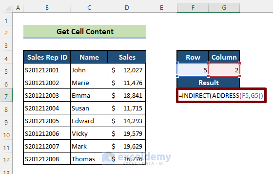
- Press ENTER.

🔎 Explanation:
- ADDRESS(F5,G5)
The ADDRESS function returns the cell address given specified the row and column number in Cell F5 and Cell G5.
Output: “$B$5”. - INDIRECT(“$B$5”)
The INDIRECT function returns the cell content in the specified cell reference, here in Cell B5.
Output: “S201212001”.
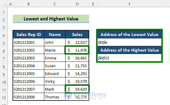
Example 5: Address of Cell with the Lowest or the Highest Value
In this example, we will see how to determine the address of the cell having the lowest or the highest value in it.
📌 Steps
- Type the following formulas in Cell F5 and Cell F7.
For the address of the Lowest Value:
=ADDRESS(MATCH(MIN(D5:D12),D5:D12,0)+4, COLUMN(D5))For the address of the Highest Value:
=ADDRESS(MATCH(MAX(D5:D12),D5:D12,0)+4, COLUMN(D5))
- Then press ENTER.
The following screenshot shows the address of the lowest and the highest values.
🔎 How Do the Formulas Work?
- MIN(D5:D12)
The MIN function returns the smallest value in the range D5:D12.
Output: 11476.
- MATCH(11476,D5:D12,0)+4
The MATCH function finds an exact match for the output “11476” (as specified by the third argument 0) and returns the relative position.
As we have placed the dataset in such a way that the first data occurs in the 5th row instead of the 1st row, we have added 4 in the formula to make up for this.
Output: 2+4.
- COLUMN(D5)
The COLUMN function returns the column number of the specified cell reference in its argument.
Output: {4}. - ADDRESS(6,{4})
Finally, the ADDRESS function returns the cell address with respect to the specified row and column numbers returned by the other functions, MATCH, and COLUMN.
Output: {“$D$6”}.
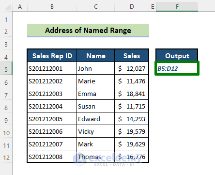
Example 6: Get the Address of a Named Range
To demonstrate this example, let’s first create a named range, “Data” just like the following screenshot. To learn how to create a Named Range, click here.
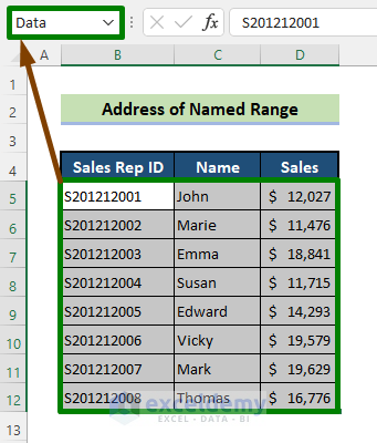
Now, if we want to get the full address of the named range “Data”, we need to follow the steps below.
📌 Steps
- First of all, type the following formula in Cell F5:
=ADDRESS(@ROW(Data),@COLUMN(Data),4)&":"&ADDRESS(@ROW(Data)+ROWS(Data)-1,@COLUMN(Data)+COLUMNS(Data)-1,4)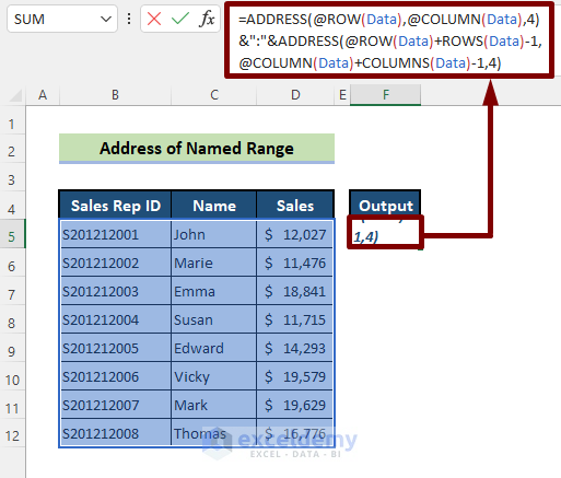
- Press ENTER.
The following picture shows the address of the named range “Data”.
Note:
- In Excel 2021 and 365, we have to use the Implicit Intersection Operator (@) before the ROW and the COLUMN function in this formula so that the formula doesn’t behave like an array formula and returns a single output.
- If you use Excel 2019 or an earlier version of Excel, just wipe out the @ sign from the formula and press ENTER.
🔎 How Does the Formula Work?
- @ROW(Data) and @COLUMN(Data)
In Excel 365, ROW(Data) would return {5;6;7;8;9;10;11;12} and COLUMN(Data) would return {2,3,4}.
As we need only the first number in the array, we have added the implicit intersection operator and the output will be the following.
Output: 5 and 2.
- ADDRESS(5,2,4)
The ADDRESS function returns the cell address in relative reference style.
Output: “B5”.
- ROWS(Data) and COLUMNS(Data)
These functions return the number of rows and columns in the Named Range “Data”.
Output: 8 and 3.
- ADDRESS(@ROW(Data),@COLUMN(Data),4)
This part of the formula returns the address of the first cell of the range.
Output: “B5”.
- ADDRESS(@ROW(Data)+ROWS(Data)-1,@COLUMN(Data)+COLUMNS(Data)-1,4)
This part of the formula returns the address of the last cell of the range.
Output: “D12”.
- “B5″&”:”&”D12″
Finally, the ampersands (&) concatenate the two outputs with the colon and return the final output.
Output: “B5:D12”.
Read More: How to Get Cell Value by Address in Excel
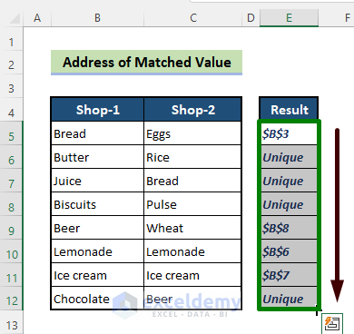
Example 7: Compare Two Columns and Get the Address of the Match
We can also use the ADDRESS function to get the address of the matched values. To do that, we have to combine the IF, ISERROR, and MATCH functions with the ADDRESS function. We will use the sample dataset-3 where there is some product data of two shops. We have to find the matches and their cell addresses. Let’s see the following steps.
📌 Steps
- First, type the following formula in Cell E5 and press ENTER.
=IF(ISERROR(MATCH(B5,$C$5:$C$12,0)),"Unique",ADDRESS(MATCH(B5,$C$5:$C$12,0),2))
- Then pull the Fill handle icon all the way.
🔎 How Does the Formula Work?
- MATCH(B5, $C$5:$C$12,0)
The MATCH function finds the match in the range C5:C12 for the content in Cell B5 and returns the relative position of the exact match in C5:C12.
Output: 3.
- ADDRESS(3,2)
The ADDRESS function returns the cell address of the cell where the 3rd row and the 2nd column intersect. We can put the column number as 2 as it is hardcoded in the formula.
Output: “$B$3”.
- IF(ISERROR(MATCH(B5, $C$5:$C$12,0)),”Unique”, MATCH(B5, $C$5:$C$12,0),2)
If the MATCH function returns #N/A, then it is tested by the ISERROR function, which returns TRUE or FALSE. The IF function returns “Unique” if the statement is TRUE and if FALSE returns the Cell Address.
Output: $B$3, Unique, Unique, Unique, $B$8, $B$6, $B$7, Unique.
Read More: How to Return Cell Address Instead of Value in Excel
💡 Things to Keep in Mind
- Please be careful and write valid arguments in the ADDRESS function.
- Invalid arguments like row or column number less than 1 or greater than the number facilitated by Excel, any non-numeric input for row_num, column_num, or [abs_num] arguments will return #VALUE! error.
- [a1] Logical input should be one of the recognized inputs provided by Excel.
Download Practice Workbook
Click on the following button and download the sample workbook to practice along with it.
Conclusion
So, we have discussed everything about the Excel ADDRESS function. If you have any confusion or questions, please feel free to ask us in the comment box. Also, let us know if you find the article useful.
Excel ADDRESS Function: Knowledge Hub
- How to Use Cell Address in Excel Formula
- Example of Cell Address in Excel
- How to Copy Cell Address in Excel
- How to Return Cell Address of Match in Excel
- Excel VBA to Find Cell Address Based on Value
<< Go Back to Excel Functions | Learn Excel

