Excel Intersection (Ranges, Named Ranges & Datasets)

In this article, we’ll focus on the topic of Excel intersection. We will explore different scenarios where this functionality works successfully. We’ll see this for single and multiple rows and columns, named ranges. We will discuss using formula and VBA macro to achieve these.

You can apply this knowledge to your real-life practical work like data analysis, market research, project management or to understand Venn diagrams also. It can help you gain insights and streamline the process more easily.

So, go through the entire article to understand the topic clearly.

Download Practice Workbook

Intersection Operator in Excel

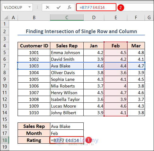
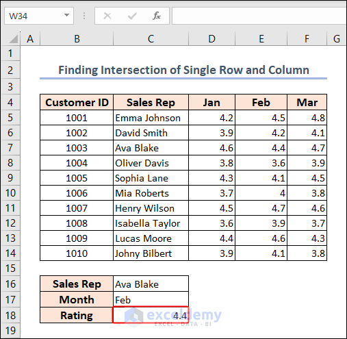
1. Find Intersection of Single Row and Column

• For finding the rating of Ava Blake in February, the formula in cell C18 is the following.

Here, the space between these two ranges in the formula works as the intersection operator.

• Press ENTER and match the output with the dataset.

Read More: Intersection of Row and Column in Excel

2. Identify the Intersection of Multiple Rows and Columns in Excel

• You can find the ratings of Ava Blake for January and February by using the following formula in cell C18.

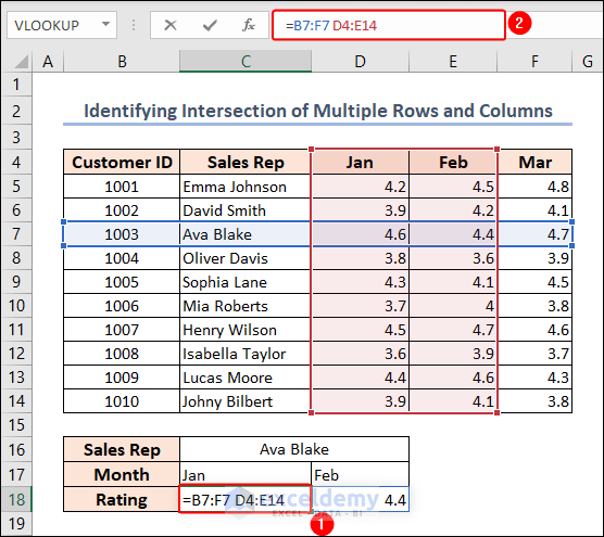
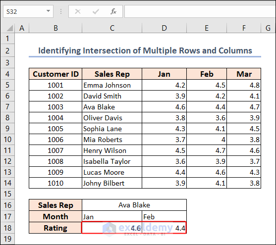
• Press ENTER and see the output. It returns two outputs as it’s an array formula.

3. Extract the Intersection of Named Ranges in Excel

In this worksheet, there are two named ranges for our example. One is SalesRep_Ava (B7:F7), and the other one is Month_Feb (E4:E14).

• Write the following formula in cell C18 and press ENTER.

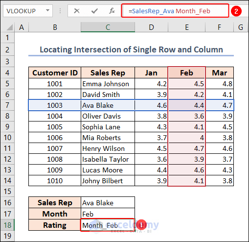
Here we get the output by using the named ranges only. We didn’t need to mention the range of cells here.

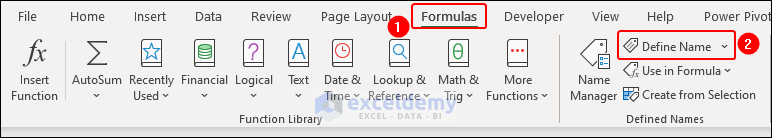
Steps to Create Named Range:

• Go to the Formulas tab >> Define Name option on the Defined Names group of commands.

• In the New Name dialog box, write SalesRep_Ava in the Name box. Then, set the Scope to this worksheet whose name is Intersection Named Range, and give B7:F7 range as cell reference in the Refers to box. Lastly, click OK.

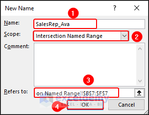
These steps will create a named range.

• Select the name from the Name Box and Excel will show its range automatically.

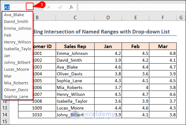
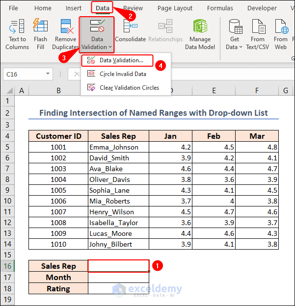
4. Find the Intersection of Named Ranges with Drop-Down Lists in Excel

• Select cells in the C4:F14 range. Then, click on Formulas >> Create from Selection.
• In the Create Name from Selection box, check the boxes of the Top row and Left column options and click OK.

• In the Name Box, you can find the newly created named ranges.

• Select cell C16. Then click on the Data tab >> Data Validation dropdown >> Data Validation option.

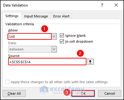
• In the Data Validation box, select List in the Allow box. Write the C5:C14 range as Source and click OK.

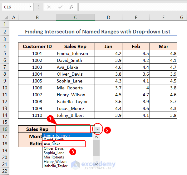
• Similarly, create another dropdown in cell C17 for the month.
• Now, select cell C16 and click on the dropdown arrow beside it. From the list, select Ava_Blake. In like manner, select the month Feb in cell C17.

• Insert the following formula in cell C18 and press ENTER.

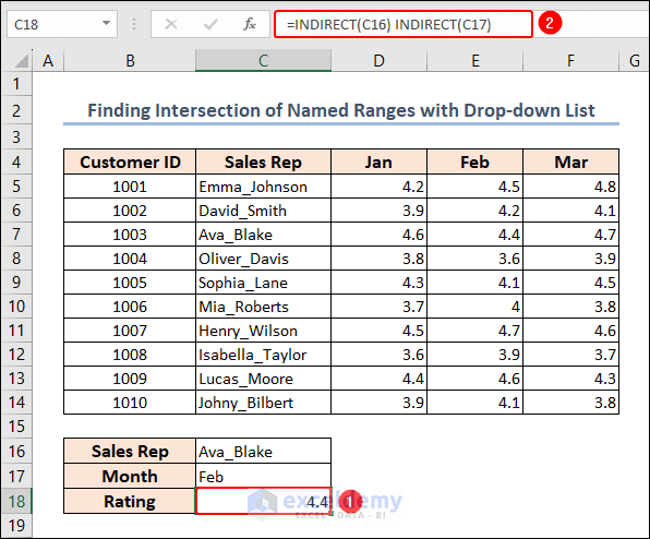
Find the Intersection of a Dataset in Two Columns

1. Combining of IF and MATCH Functions

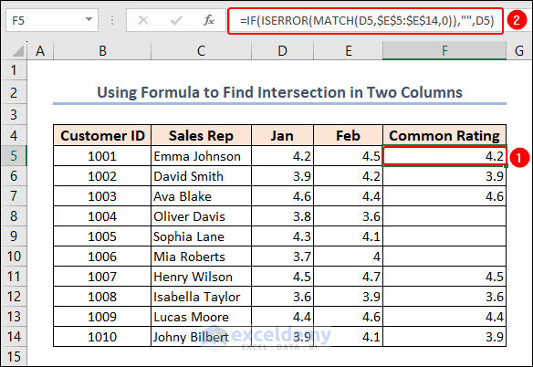
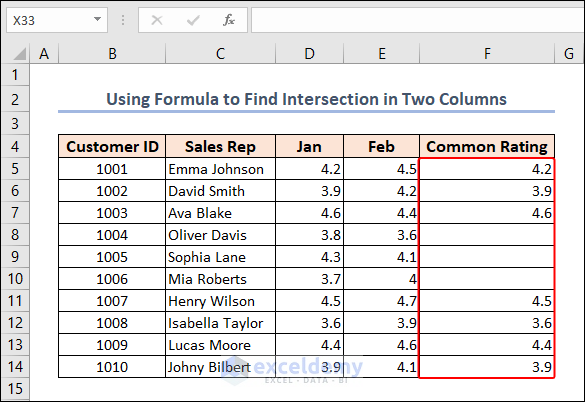
Let’s find which ratings are common in both January and February and are present in the Common Rating column.

• The formula in cell F5 is the following.

2. Apply VBA Code

• Move to the Developer tab, then click on the Visual Basic button in the Code group.

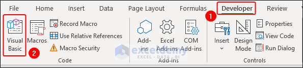
It launches the Microsoft Visual Basic for Applications window.

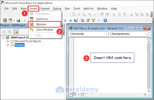
• Now, click the Insert tab and choose Module from the list. We get a small Module window to insert our VBA code.

• Here’s the working code to do the task. Paste this code into the module.

Sub Intersection_Two_Columns()
Dim Intrsctn As Variant, a As Variant, b As Variant
Set Intrsctn = Range("E5:E14")
For Each a In Selection
For Each b In Intrsctn
If a = b Then a.Offset(0, 2) = a
Next b
Next a
End Sub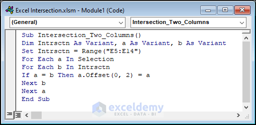

• Return to the worksheet and select cells in the Jan column (D5:D14). Then, go to the Developer tab >> Macros option.
• In the Macro dialog box, there is only one VBA macro available and selected already. Just click on Run.

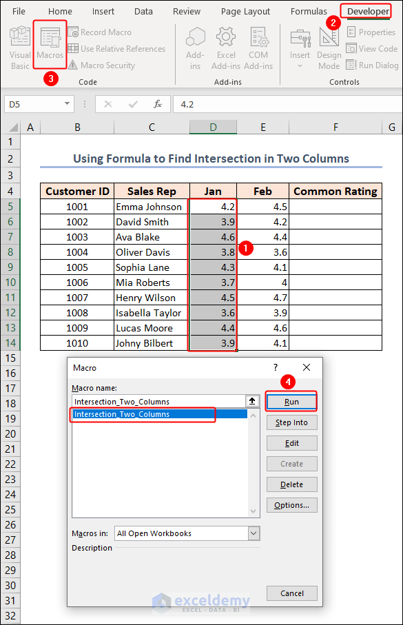
That’s the final output.

Use Implicit Intersection Operator (@) in Excel

You can calculate the total rating for the 3 months and get the result in a single cell.

• In cell G5, write the following formula.

As it’s an array formula, Excel automatically returns the output in cells in the G6:G14 range also.

But, what if you want only the result for the first row of 1001 Customer ID with the same formula?

• Simply, add the implicit intersection operator (@) before every range. The formula in cell H5 is the following.

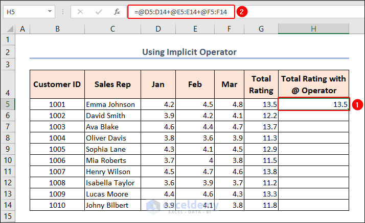
You can see that now it’s not working like an array formula. Because this operator disables the array behavior of the formula in Excel 365.

Read More: Use Implicit Intersection Operator

Things to Remember

• When creating named ranges from selection, Excel places an underscore if there is a gap between two words. So be cautious about this.
• If you use any other version of Excel except Excel 365, press CTRL + SHIFT + ENTER instead of just pressing ENTER to make array formulas work.
• In the case of the VBA method, make sure to select the range before running the macro.

Conclusion

Throughout this exploration of Excel intersections, we have tried to cover the usage of intersecting operator for single row and column, for multiple rows and columns. We also discussed it in the case of named ranges and also with drop-down lists.

Rather than that, we showed how we can use the formula and VBA macro to find the intersection of the dataset in two columns.

So, that’s all for today. If you have any questions, comments, or recommendations, kindly leave them in the comment section below.

Frequently Asked Questions

1. Is there a built-in function in Excel for finding intersections?

Excel does not have a specific built-in function for finding intersections. However, you can achieve the same result using formulas or features.

2. Can I highlight the intersecting values in Excel?

Yes, you can highlight the intersecting values in Excel using conditional formatting.

3. How can I count or sum values at an intersection?

You can use COUNTIFS or SUMIFS functions to count or sum values at an intersection based on specific criteria or conditions.

Excel Intersection: Knowledge Hub

• Use Intersection Operator
• Performing Intersection of Two Data Sets
• Intersection of Two Columns

<< Go Back to Excel Operators | Excel Formulas | Learn Excel