How Can You Alternate Row Colors in Excel? (4 Easy Ways)

Get FREE Advanced Excel Exercises with Solutions!

In this Excel tutorial, we will show you how to apply alternating row colors in Excel using a manual approach, conditional formatting, table formatting features, and VBA code.

While preparing this article, we used Microsoft 365 for applying all operations, but they are also applicable in all Excel versions.

In Excel, alternating row colors is a helpful formatting trick that enhances data organization and readability. You can quickly distinguish between various sets of information by alternating the row colors.

Download Practice Workbook

Alternating Row Colors.xlsm

Table of Contents Expand

How to Apply Alternate Row Colors in Excel?

There are 4 different ways available to alternate row colors. You can alternate row colors by manually selecting the rows, using preset table styles, applying conditional formatting, or embedding VBA macro in Excel.

Let us see how these methods work.

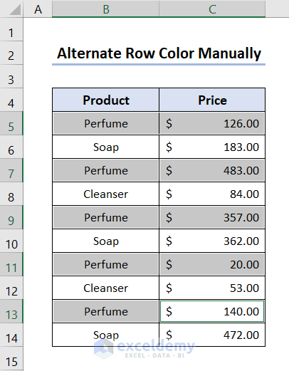
1. Applying Alternate Row Color Manually

You can alternate row colors by manually selecting the cells and applying the fill color to them. Let’s see the steps to apply alternate row colors manually.

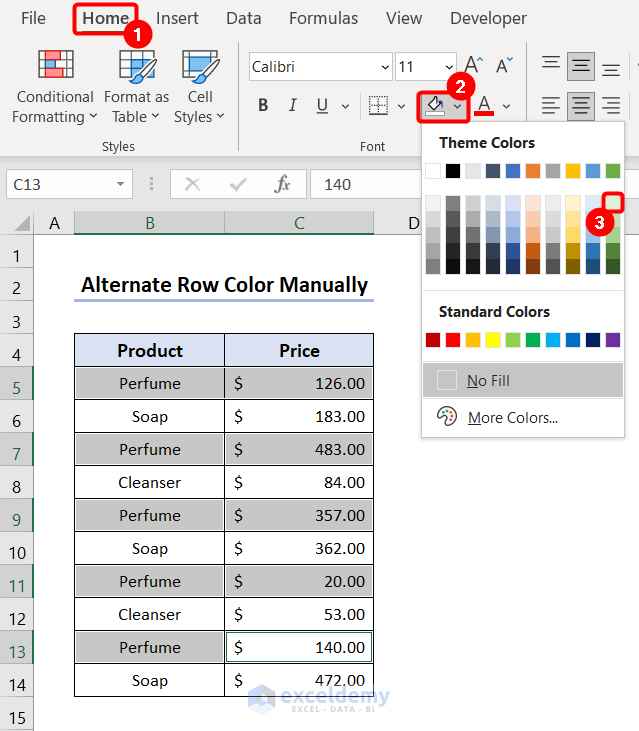
Select the alternate rows by clicking on them while holding down the Ctrl key.

Then go to the Home tab and click the Fill Color option from the Font group.
There are Theme Colors and Standard Colors. You can choose any color according to your desire. We chose Green, Accent 6, and Lighter 80% from the Theme Colors.

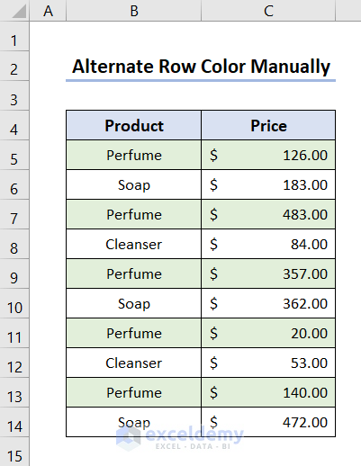
We will now have alternate rows colored in Excel.

If you have a large dataset, then this method might become hectic. In that case, follow the steps below.

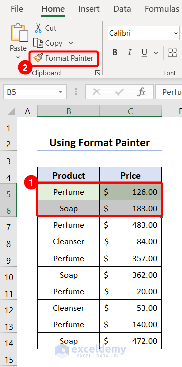
Select the first row and apply Fill Color from the option in the Home tab.

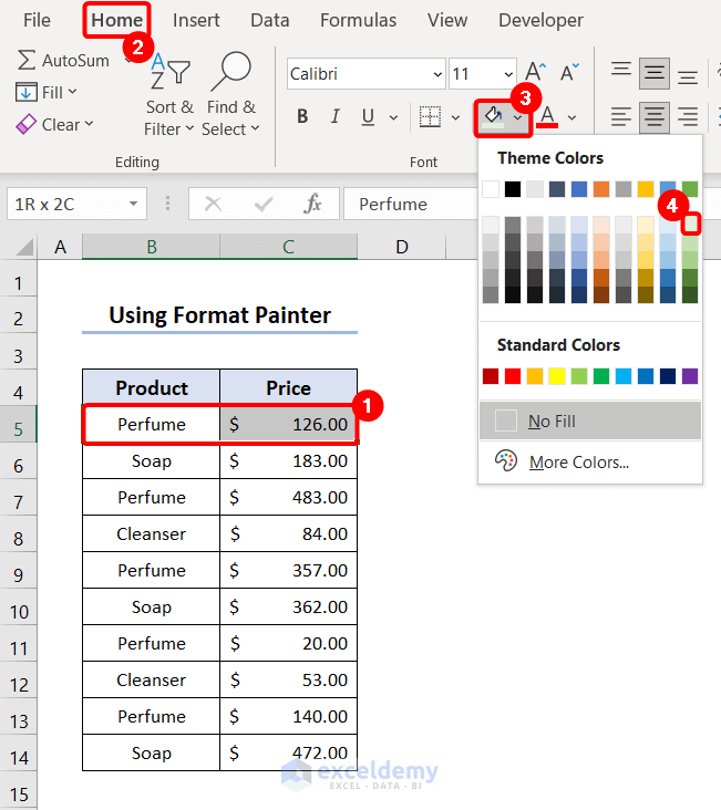
Next, select the colored row and the row below it.
Click on Format Painter from the Clipboard group in the Home tab.

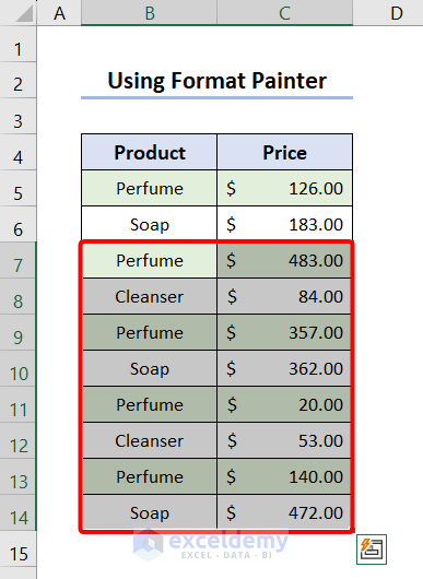
Then, select all the other rows, and this format will be painted on them. Thus, we will get rows colored alternately.

2. Using Preset Table Format for Alternating Row Color

A preset table style is one of the simplest ways to color rows alternately. Let’s see how to use them.

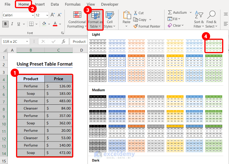
Select the dataset you want to color alternately by rows.
Then, choose a table style on Format as Table from the Home tab. We chose a Green banded table from the Light option.

Selecting table style from format table option

Click the image to see the full view.

Next, ensure that the My table has headers option is checked in the Create Table box and press OK.

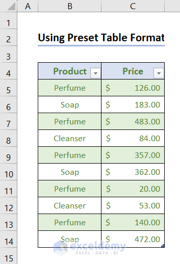
Now, you will see the dataset formatted as a table and rows colored alternately.

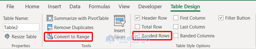
If you want to customize this table, select the table, go to the Table Design tab, and customize from the options.
Also, if you do not want a table, only want the format, then from the Tools option, click on Covert to Range. The table will transform into ranges.

Click the image to see the full view

3. Applying Conditional Formatting for Coloring Rows Alternately

Yes, you can apply alternating row colors using Conditional Formatting.

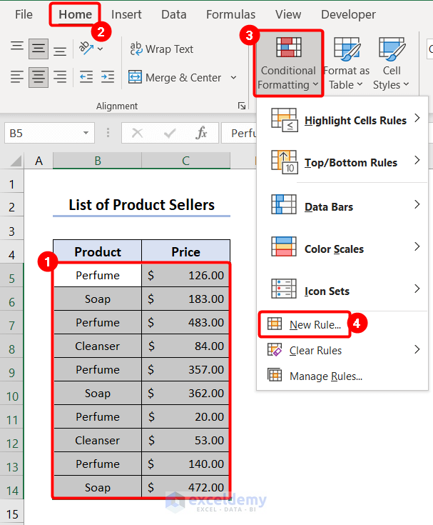
To do this, select the cells where you want to apply formatting.
Click Conditional Formatting from the Styles group in the Home tab and select New Rule.

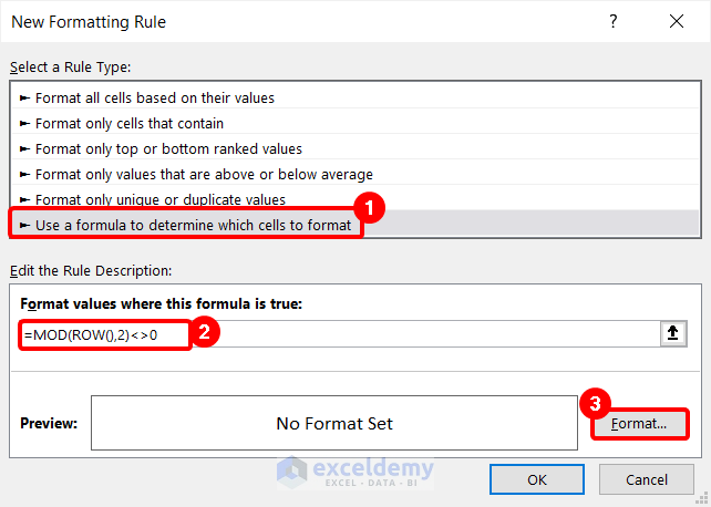
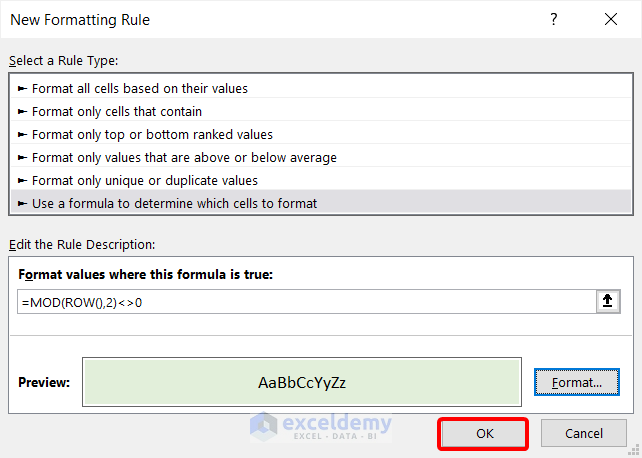
Now, click on Use a formula to determine which cells to format, insert the formula below in Format values where this formula is true, and click on Format.

=MOD(ROW(),2)<>0

Here, we wanted to apply color to the odd-numbered rows. This formula divides the row number by two, then returns true if the remainder is not equal to two.

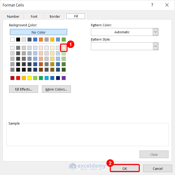
N.B.: If you want to apply color to even-numbered rows, then change the not equal to (<>) sign into an equal (=) sign. Besides, you can apply ISEVEN and ISODD functions along with ROW functions for consecutively coloring even and odd-numbered rows.

Now, from the Format Cells box, choose Fill, click on any color you choose, and press OK.

Now press OK, and you will have the odd-numbered rows colored.

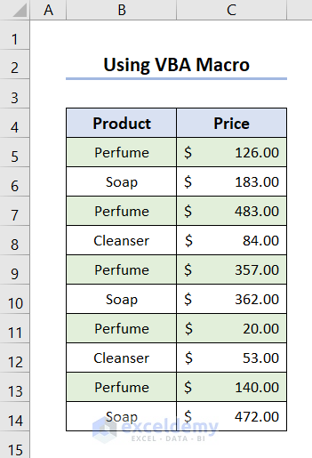
4. Alternating Row Colors Using VBA Macro

You can alternate row colors using a VBA macro. Let’s see the macro for alternating row color.

First, select Visual Basic from the Developer tab to embed a Macro.

Then, a named box for Microsoft Visual Basic for Application will appear. Choose Module from the Insert tab.

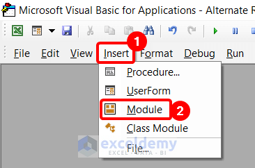
Now, in the module, insert the code below.

Sub AlternatingRowColors()
Dim R As range
Dim row As Long
Dim NoCol As Long
Dim Color As Long
  NoCol = vbWhite
  Color = RGB(226, 239, 218)
  Set R = Selection
  If R.Rows.Count = 1 Then Exit Sub
  For row = 1 To R.Rows.Count
    If row Mod 2 = 0 Then
      R.Rows(row).Interior.Color = NoCol
    Else
      R.Rows(row).Interior.Color = Color
    End If
  Next row
End Sub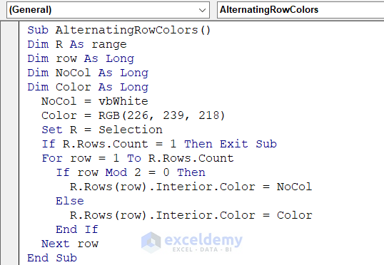

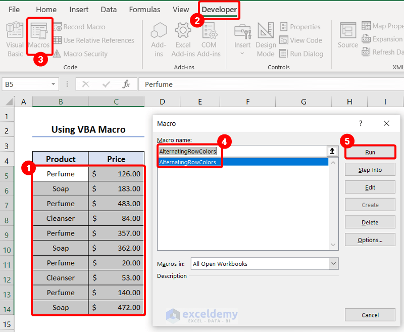
Now go back to the sheet, select the range, click on Macros in the Developer tab, or press Alt+F8.
Next, choose AlternatingRowColors and click on Run.

Click the image to see the full view

The alternate row colored data looks like this.

Which Things You Have to Keep in Mind?

While applying Conditional Formatting, select the formatting options by clicking the Format button after creating the formula. For the alternating rows, you can choose your preferred fill color.
Use a dynamic range in the conditional formatting formula if you want the formatting to change automatically when new or removed rows are added or removed. For instance, to cover a wider range, you can use a formula like $A$2:$A$100 instead of choosing a smaller fixed range like A2:A10.
While applying macro, ensure you have the Developer tab. If you do not have this tab, go to the File tab and click Options. Then from the Excel Options, go to Customize the Ribbon and put a check on the Developer option.

Frequently Asked Questions

1. How to remove Excel’s alternating row colors?

Answer: First, select the cells or the table to which the alternating row colors will be applied. Go to the Styles group under the Home tab. Choose Clear Rules from the drop-down menu under the Conditional Formatting button. Now, to remove the alternating row colors from the selected range, select Clear Rules from Selected Cells.

2. How do I apply alternating row colors to a part of my data?

Answer: To apply alternating row colors to a part of your data, instead of selecting the entire table, you can select a specific row or a set of cells to apply the alternating row colors to and apply the color or formatting using Conditional Formatting or Fill Color.

3. Does Excel’s data change when row colors alternate?

Answer: Alternating row colors in Excel is a visual formatting feature. The alternating colors are only used to improve visual distinction and readability; the data does not change.

Conclusion

This article includes different methods for alternating row colors in Excel. You can alternate row colors quickly using Excel conditional formatting or formatting as a table feature. Moreover, row colors can be altered by inserting various formulas and VBA macros. Besides, you can manually color the alternate rows, too.

These methods simplify interpreting and analyzing data, making it especially helpful when working with large datasets or complicated tables. You can effectively present your information and increase user accessibility using alternating row colors. Use these Excel techniques to improve your data’s readability and visual appeal and simplify your data analysis tasks.

Alternating Row Colors in Excel: Knowledge Hub

<< Go Back to Highlight Row | Highlight in Excel | Learn Excel