Excel Table (Insert, Customize, and Applications)

Get FREE Advanced Excel Exercises with Solutions!

In this Excel tutorial, we will learn in detail about Excel table including inserting, customizing, and using multiple features.

An Excel table is known as a data container used for storing data that can sort, filter, and analyze data. It’s an all in all solution for handling data and making spreadsheet tasks easy and dynamic.

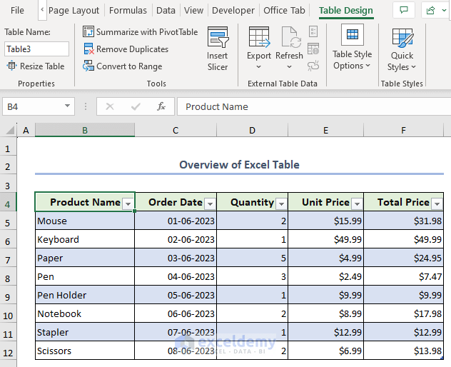
In the following, you will find an overview of Excel table. We used Microsoft 365 to prepare this article. But you can apply the operations in Excel versions from Excel 2007 onwards.

Download Practice Workbook

Download the workbook that we used to prepare this article.

Excel Table.xlsx

Table of Contents Expand

What Is Excel Table?

An Excel Table is a structured range of data within Excel that offers various advantages. It is a collection of related data organized in rows and columns with a designated header row. Built-in features like automatic expansion of formulas, easy sorting and filtering options, and dynamic named ranges make it one of the top features in Excel.

How to Insert an Excel Table

1. Using Insert Option

Simply, select any cell (E9) from the table in your worksheet.
Click the Table option from the Insert tab.

Next, choose your desired cell range and hit OK.

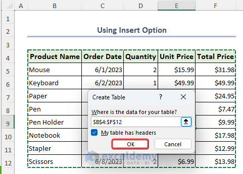
As a result, you will get your table inserted for the chosen cell range.

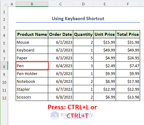
2. Using Keyboard Shortcut

Select any cell from the range.
Then just press CTRL+L or CTRL+T, to create your Excel table within a glimpse.

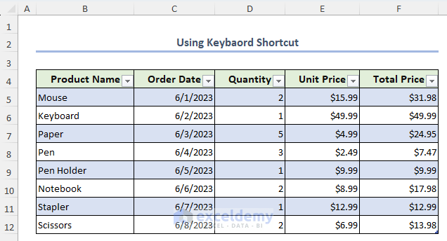
Finally, you will get your Excel table in your hand.

How to Customize an Excel Table

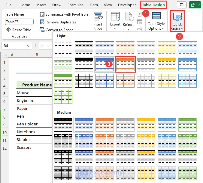
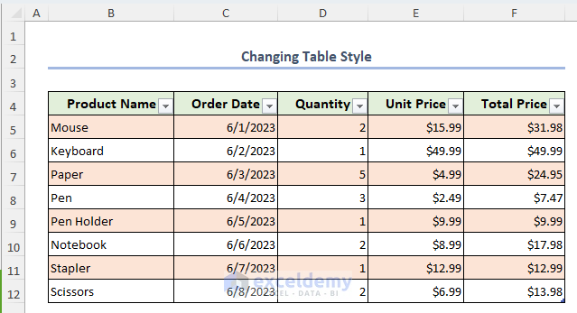
1. Changing Table Style

If you want you can change the color of rows and columns in a table.

First, choose any cell from the table and then visit the Table Design feature.
Second, from the Quick Style option choose your desired color.

As a result, we have successfully customized our table with our desired color.

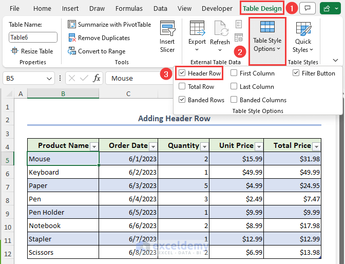
2. Adding Header Row

Similarly, for working advantages, you can add or remove the header row. For this,

Remove the checkmark from the Header Row option lying in Table Style Options.

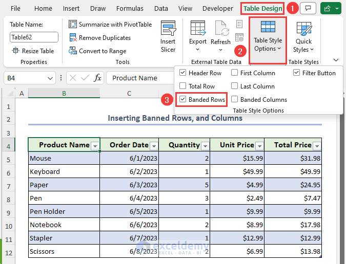
3. Inserting Banned Rows, and Columns

To get the banned color for the columns checkmark the Banded Columns from the Table Design feature.

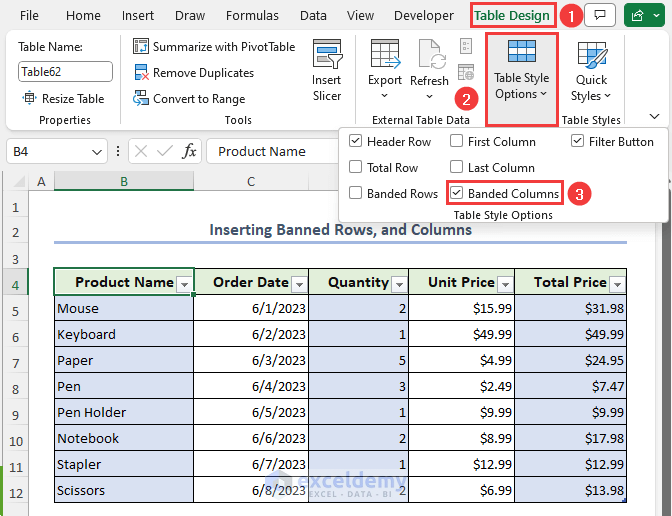
In the same fashion, checkmark the Banded Rows option to insert color for the rows.

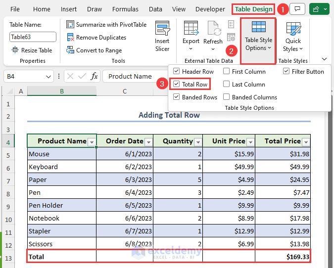
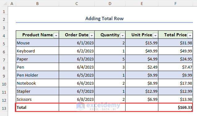
4. Adding Total Row

When you have to handle a larger dataset, you need the total value at the end location. For that, the Excel table has also introduced three quick ways to get the Total Row feature.

Simply, add the Total Row from the Table Design option.

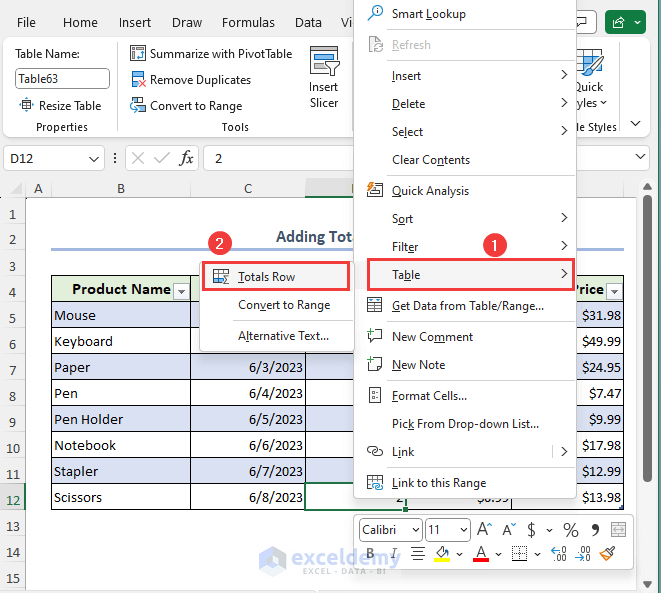
You can also operate the advanced options by right-clicking the mouse button.
Then click the Totals Row from the Table option.

Pressing CTRL+SHIFT+T will also lead to adding the total row in a table.

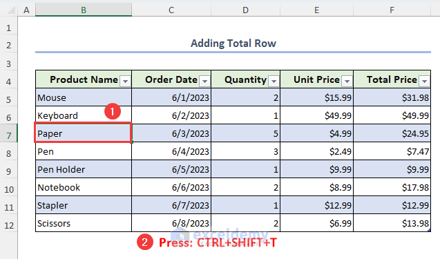
By operating the actions above you will get the total row added in your Excel table. It’s that simple.

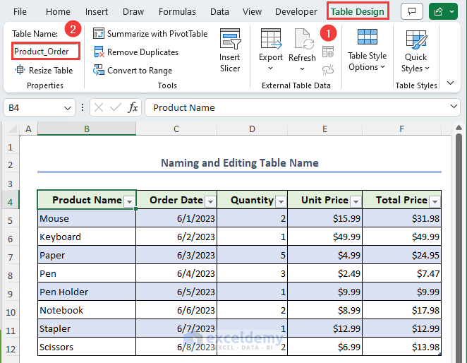
5. Naming and Editing Table Name

If you want to call your table in another worksheet then you must name your table.

For that, visit the Table Design feature and provide a name in the Table Name section.

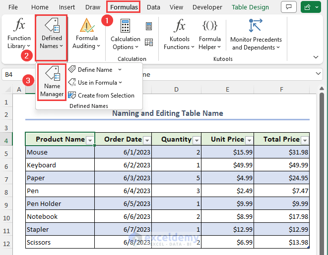
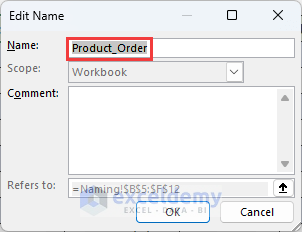
In order to change the table name you can visit the Name Manager option from the Formulas tab.

In the Name Manager window, click the Edit option.

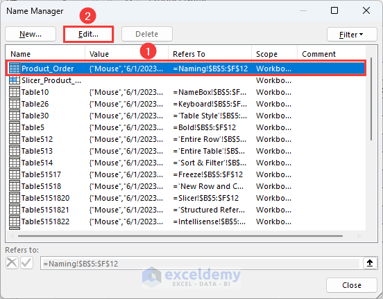
From the Edit Name window, write your desired name for the table to change to the final Excel table name.

Read More: Table Name in Excel

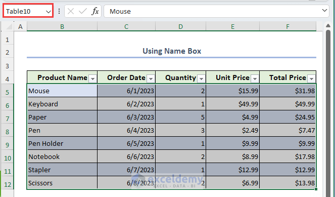
6. Using Name Box

To directly travel to your desired Excel table you can utilize the Name Box list.

Opening the workbook, open the drop-down list from the Name Box, and choose your desired table name.

According to the selection, you will directly jump to the Excel table.

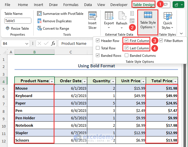
7. Using Bold Format

Visit the Table Design feature and checkmark the First Column and Last Column to bold all the data from the first and last columns.

How to Use an Excel Table

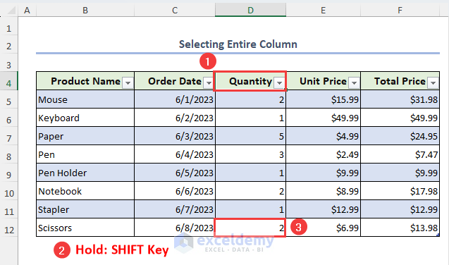
1. Selecting Entire Column

With a large dataset, you may face problems with selecting the entire column. Here I have shared some simple tricks to select an entire column within seconds.

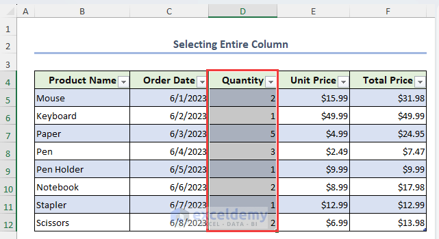
Select a cell (D4) from the top.
Press CTRL+SPACE or CTRL+SHIFT+Down Arrow(↓) to choose the entire column from a table.

While selecting the top cell (D4) from a table, hold the SHIFT key and then click the last cell (D12) of the same column to select the entire column.

Select a header cell (D4) from a table and move the mouse cursor to get the icon just like the image below.
When the icon appears, left-click the mouse button to select the whole column.

You can also click the Table ColumnData from the Advanced options appearing by right-clicking the mouse button.

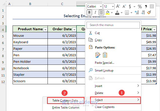
Following these above steps you will get to see the entire column is selected from the Excel table.

2. Selecting Entire Row

In order to select the entire row you can use keyboard shortcuts or advanced options.

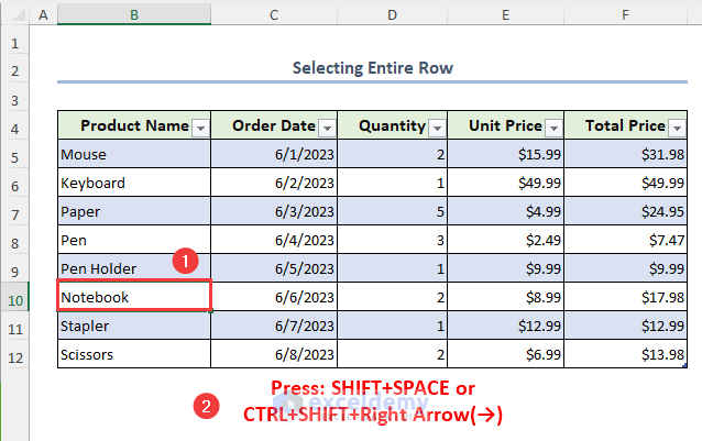
Select a cell (B10).
Press SHIFT+SPACE or CTRL+SHIFT+Right Arrow(→) to choose the entire row.

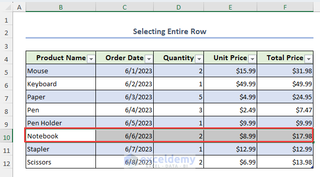
Choosing a cell (B10), hover the mouse over the cell border to get the icon just like the below image.
When the sign appears, click the left button of the mouse to choose the entire row.

Choose the first cell (B10).
Holding the SHIFT key choose the last cell (F10) from the same row to select the entire row.

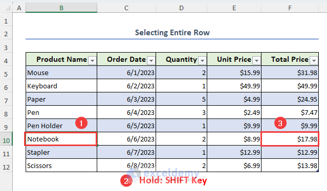
Visit the Advanced options by clicking the right button of the mouse and click the Table Row to select the entire row.

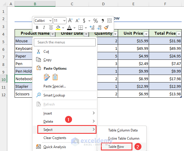
Following the above steps you will see the entire row is selected just like the below image.

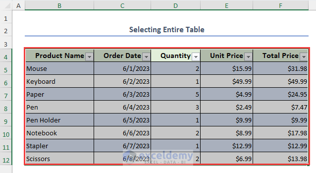
3. Selecting Entire Table

First, select the top left cell (B4).
Move the mouse over the border of the cell to get the icon following the image below.
When the icon appears click the left button of the mouse to select the entire table.

Thus you will see the whole table is selected except the header.

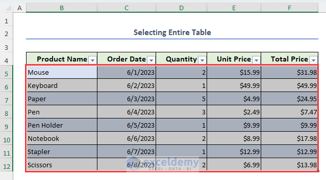
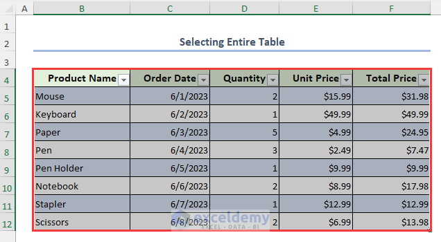
While selecting any cell from the table press CTRL+A to choose the entire table.

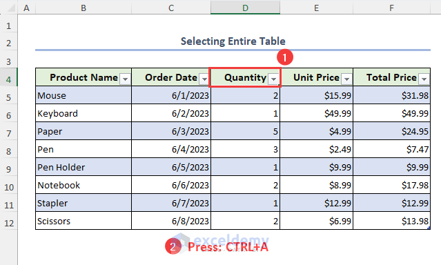
Following the footprints you will see the entire table is selected with the header.

Hover your mouse over the border of the table until you see the four-directional icon.
When the icon appears, simply press the left button of the mouse.

This way you will see the entire table is selected for the Excel table.

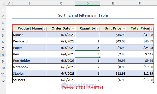
4. Sorting and Filtering in Table

For complex and large datasets you will need to utilize sorting and filtering in Excel.

Enable the sort and filter feature in the Excel table by checking the Filter Button from the Table Design tab.

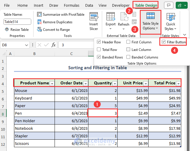
You can also utilize the keyboard shortcut by pressing CTRL+SHIFT+L to enable and disable the filter feature inside a table.

Clicking the Filter icon you will have the sort and filter window for the table.

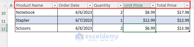
5. Freezing Column Header

For viewing a large dataset with a header while scrolling you have frozen the header row previously. But for the Excel table, you don’t need to freeze the column header as it’s automatically enabled.

Simply, choose any cell (E12) from the table and scroll down.

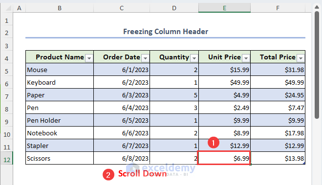
While scrolling you will see the column header is enabled for the table in Excel.

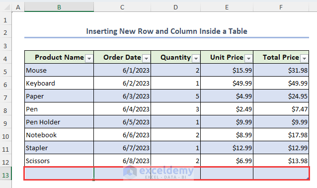
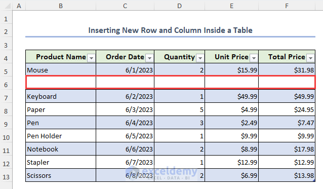
6. Inserting New Row and Column Inside a Table

After creating a table you might need to add more rows or columns for the same table. Well, in this method, I have shared some simple ways to insert new rows and columns inside a table.

To insert a new row, select the last cell (F12) from the table and press the TAB button from the keyboard.

Thus, a new row will be inserted for the table.

Insertion of a new row inside a table can also be done by choosing a cell (B6) and clicking the Table Rows Above from the Advanced options.

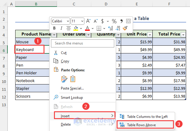
As a result, a new row will be inserted immediately above the selected cell.

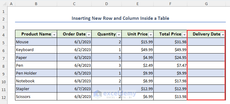
In order to insert a new column choose a cell (G4) side by side to the table, write the column heading, and hit ENTER.

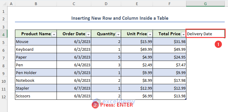
A new column will be inserted for the Excel table within a blink of an eye.

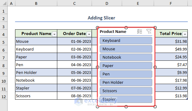
7. Adding Slicer

In order to add slicers, visit the Table Design tab and click the Insert Slicer feature.

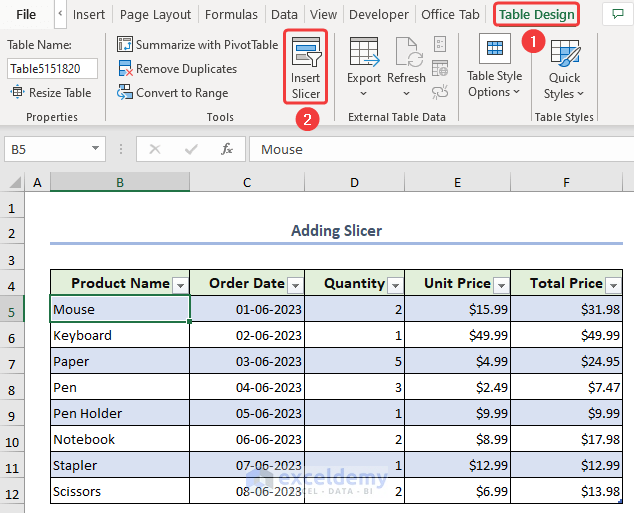
Within a glimpse, a slicer for filtering the table will be created. It’s that simple.

8. Structured Referencing

Structured referencing is a useful feature in Excel table where you will see table references instead of cell references inside a formula making it easier to understand.

Select a cell (F5) and write the below formula with table reference where structured referencing is applied for a column.

=[@[Unit Price]]

To calculate the Total Price, similarly choose a cell (F5) and put the below formula with table references.

=[@[Unit Price]]*[@Quantity]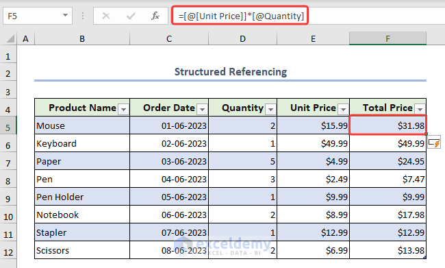

9. Applying Intellisense

What if you get to see structured references appearing while writing formulas? Won’t it be great? Well, while typing formulas intellisense menus will appear for a table.

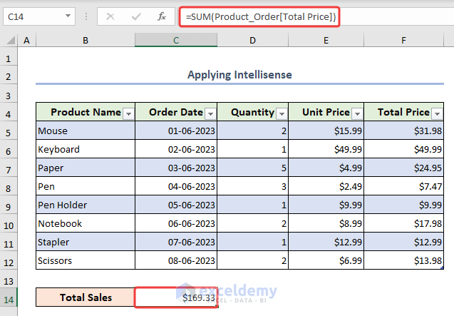
Choose a cell (C14) and write the below formula. At the time of writing you will see the intellisense menu appearing.

=SUM(Product_Order[Total Price])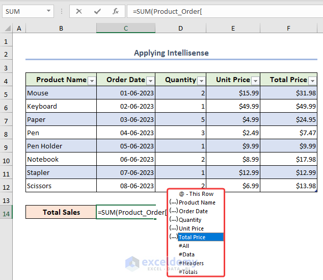

Finally, the Total Sales value will be shown inside the cell where the intellisense menu was used for saving time.

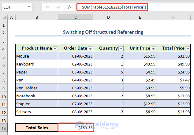
10. Switching Off Structured Referencing

While applying formulas inside an Excel table you will see the structured references instead of cell references just like the below image.

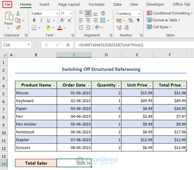
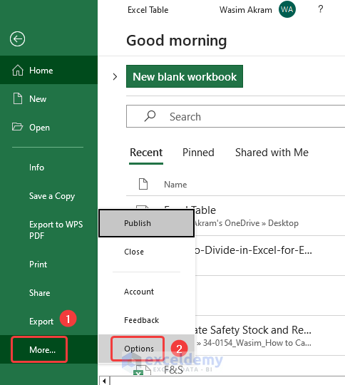
To avoid this you can turn off the structured referencing by clicking the File tab.

Now, press Options from the new window.

Hence, remove the checkmark from the Use table names in formulas option and hit OK.

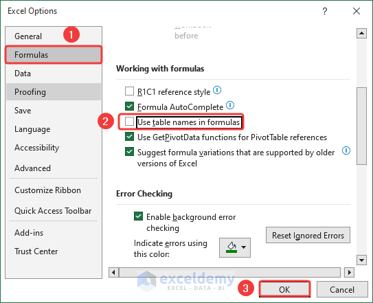
As a result, you will see the cell references while applying formulas instead of structured referencing.

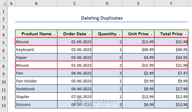
11. Deleting Duplicates

Excel table has some wonderful features where you won’t need to find duplicates one by one. Suppose we have a dataset with a duplicate inside the table.

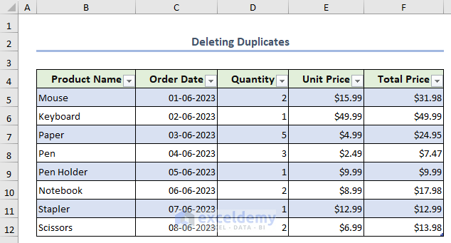
In order to delete duplicates select the Remove Duplicates option from the Table Design tab.

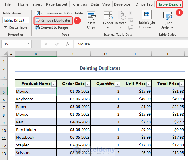
Immediately, you will see the duplicate row is removed.

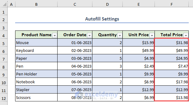
12. Autofill Settings

At the time of applying formulas inside a table you won’t need to drag down the fill handle as the filling is done by default.

Choose a cell (F5), write the below formula, and hit ENTER.

=[@Quantity]*[@[Unit Price]]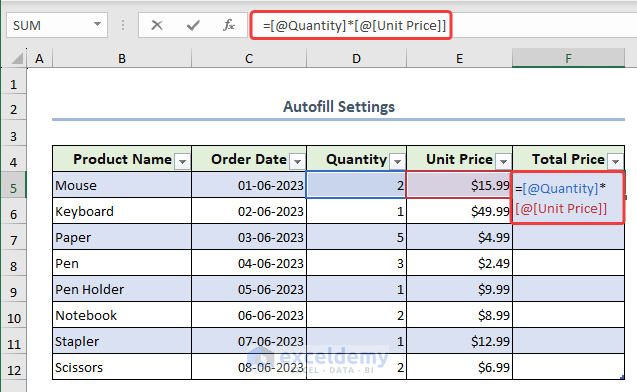

The whole column will be filled with the result.

13. Resizing Table

Sometimes you might need to resize the table contents to rearrange the data.

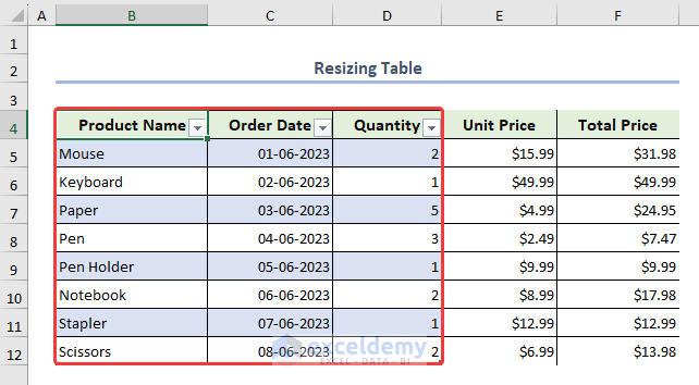
To do so, click the drag icon from the end of the table to resize.

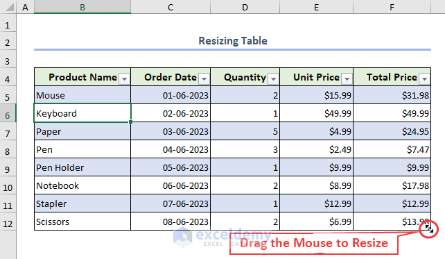
In conclusion, the table will be resized within a moment.

You can click the Resize Table option from the Table Design tab.

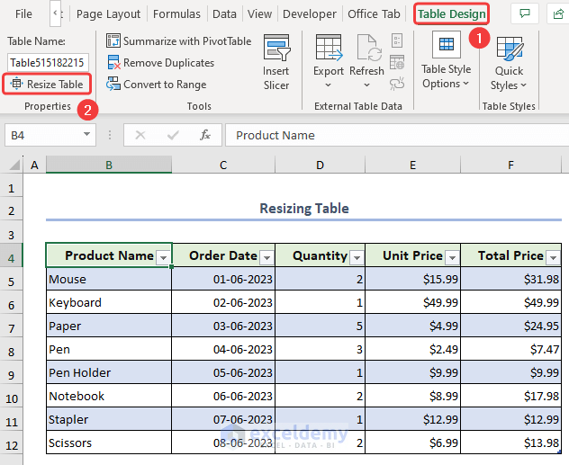
Now, put your desired range and press OK.

As a result, the table will be resized according to the provided cell range.

14. Printing Selected Area

If you want you can print the chosen area of the Excel table from the whole worksheet.

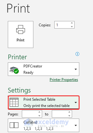
Opening the worksheet press CTRL+P to directly travel to the printing window.

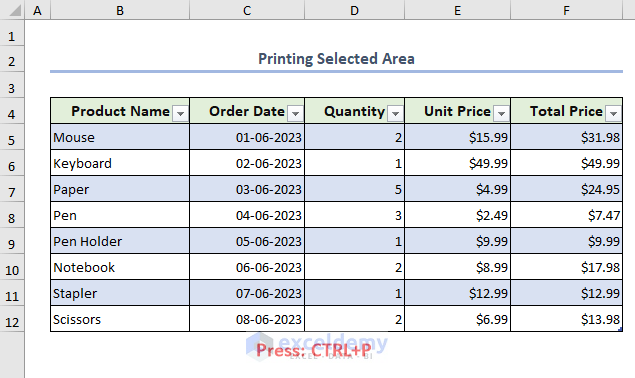
From the Settings drop-down list choose the Print Selected Table to print only the Excel table.

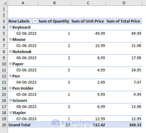
15. Summarizing a Table

To summarize the table, click the Summarize with PivotTable option from the Table Design tab.

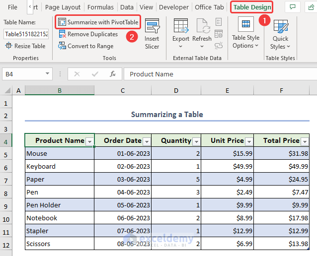
From the new window, click New Worksheet, checkmark the Add this data to the Data Model option and hit OK.

Finally, you will get the total summary of the Excel table in a new worksheet.

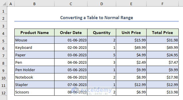
How to Convert a Table to Normal Range in Excel

For converting your table to a normal range, select the Convert to Range option from the Table Design tab.

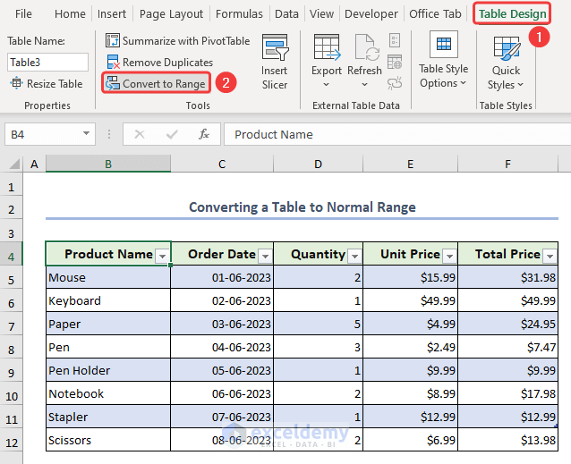
As a result, Excel has converted the table to a normal range. Simple isn’t it?

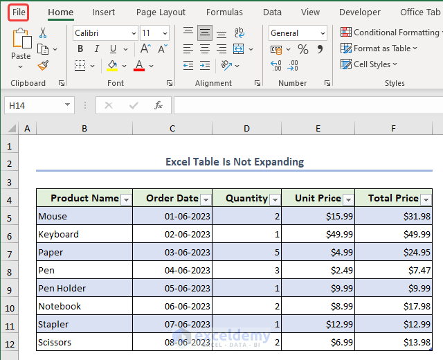
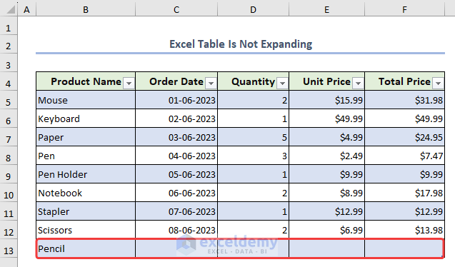
[Fixed!] Excel Table Is Not Expanding Properly

Sometimes you will see that the table is not expanding when you put new data inside it following the image.

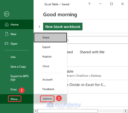
To solve this, visit the File option.

Then, choose Options from the new window.

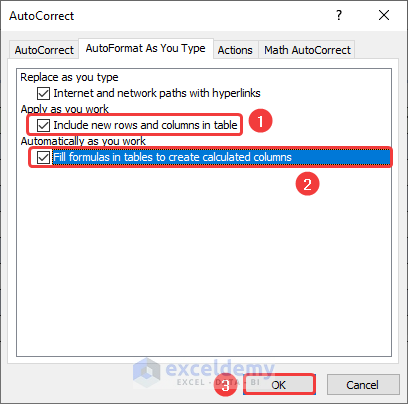
After that, click Proofing and visit AutoCorrect Options.

From the popped window checkmark the Include new rows and columns in table and Fill formulas in tables to create calculated columns option and hit OK.

Now, if you insert rows and columns inside the table you will see it’s expanding properly.

Things to Remember

While maintaining data within a table try to avoid merging cells. It can cause some problems with sorting, filtering, and data analysis.

Frequently Asked Questions

1. Is it possible to apply conditional formatting to an Excel table?

Yes, you can apply conditional formatting inside an Excel table by visiting the Conditional Formatting feature from the Home tab.

2. Can I remove the header row from an Excel table without converting it to a range?

By utilizing the Table Design tab, you can easily remove the header row from an Excel table without converting it to a range.

3. How do I remove a calculated column from an Excel table?

Simply, visit the Table Design tab, select the column, right-click the column header, and click Delete Column to remove the column from an Excel table.

Conclusion

Excel table is a powerful data organization tool that offers numerous benefits including automatic filtering, sorting, and formatting. This feature provides a structured layout, enabling easy data manipulation, and facilitating efficient data analysis. Take a tour of the practice workbook and download the file to practice by yourself. Please inform us in the comment section about your experience. We, the Exceldemy team, are always responsive to your queries. Stay tuned and keep learning.

Excel Table: Knowledge Hub

<< Go Back to Learn Excel