It is a very common occurrence to find the position of a particular character or text within a string. This is helpful for data analysis purposes such as extracting, text parsing, etc. Both FIND and SEARCH functions can be used for this purpose. However, in some cases, one can be more suitable than the other. This article will cover an in-depth analysis of the FIND and SEARCH function in Excel, their similarities and differences.
Introduction to Excel FIND Function
In Microsoft Excel, the FIND function is generally used to extract the position of a defined text in a cell containing a text string.
- Syntax
FIND(find_text, within_text, [start_num])
- Arguments
find_text is a text or a part of a text to be searched for in a cell containing another text string.
within_text is the cell containing the text where the function will search the defined character or part of the text.
[start_num] is an optional argument which is a defined position in the text string from where the character count will initiate. The default value is 1.
Introduction to Excel SEARCH Function
The SEARCH function returns the number of characters after finding a specific character or text string, reading from left to right. This function searches for a case-insensitive match. It works for both array and non-array formulas.
- Syntax
SEARCH(find_text,within_text,[start_num])
- Arguments
find_text is the text that we search for. It can be a single text or an array of texts.
within_text is the value within which the function searches for the find_text argument. It can be a single text value or an array of text values.
[start_num] is an optional argument like the one used in the FIND function. It is the position of the within_text argument from which it starts searching. It can be a single number or an array of numbers. The default value is 1.
FIND and SEARCH Function in Excel: 2 Comparison Studies
As we can see from the previous sections, both the FIND and SEARCH functions serve the same purpose. They have the same arguments, even the default optional one. However, there can be different results in some cases. This section will cover the different outcomes and their cause for the functions.
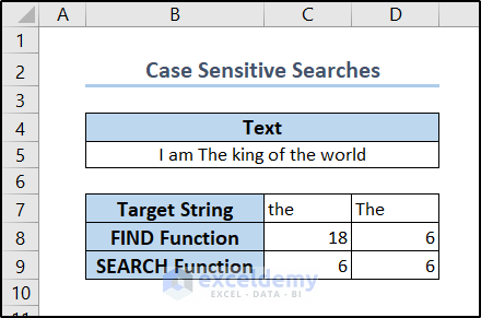
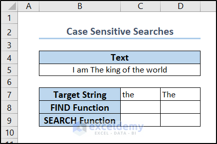
1. FIND and SEARCH Function Application for Case Sensitive Searches
This is the main difference between the FIND and SEARCH functions in Excel.
Let’s take the following dataset for the demonstration. The dataset contains the text “I am The king of the world”. There are two “the”s in the string. One has an uppercase “T” at the start.
- Insert the following formula in cell C7. You will see the position of the string “the” is 18.
=FIND(C7,B5)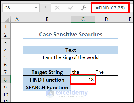
- If we insert the following formula instead, we will see the position of the string is 6.
=FIND(D7,B5)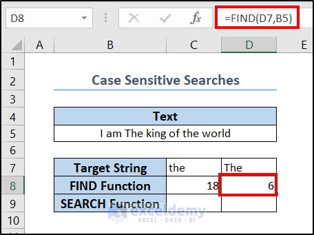
- For the SEARCH function, insert the following formula. The position of the string here is 6.
=SEARCH(C7,B5)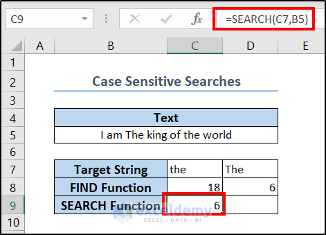
- If we insert the following formula for capitalized letters, we can see that the function, once again, gives the result 6.
=SEARCH(D7,B5)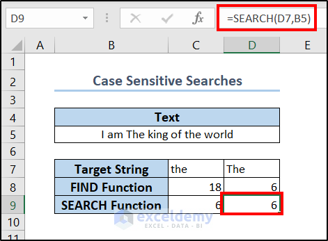
As we can see, when we search for the string “the”, the FIND function will give us the value of the one with the lowercase letter. This is the starting position of “the” before the “world”.
While searching for “The” with the FIND function it gives 6 which is the starting position of “The” before the “king”.
Irrespective of “the” or “The” we put inside to find with the SEARCH function, we get 6. Because this always targets the one before the ‘king” and is the first match.
2. FIND and SEARCH Function with Wildcard Arguments
Another major difference between the FIND and SEARCH functions in Excel is the ability to search with wildcard arguments.
Let’s take the following dataset. It contains some sentences informing about book publishing years. We are going to search if the years in the 20th century are available in the dataset.
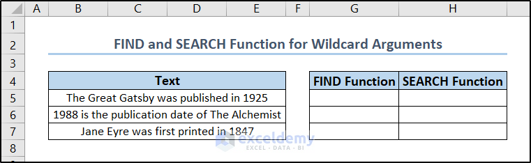
The search string we are going for is “19**”. It searches for any string that starts with 19 and will give us the position where 1 starts here if there is a match in the string. Let’s see how it interacts with FIND and SEARCH functions in Excel.
- Inserting the following formula in cell G5 and filling it in G7 gives us an error.
=FIND("19**",B5)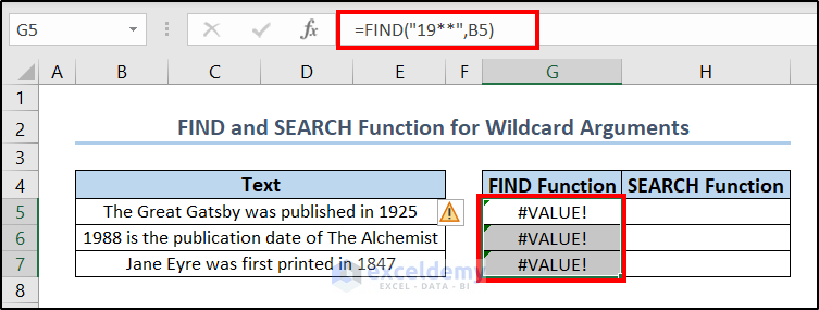
- If we use the following formula for the range H5:H7, we will get some results.
=SEARCH("19**",B5)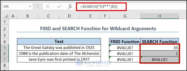
Although there are some matches in the first and second strings, the FIND function will always result in a #VALUE error. However, the SEARCH function can pick up the values and returns the position where it found the match. Only the third one gives an error because the year specified in cell D7 does not meet the criteria.
This is another thing to consider while distinguishing between FIND and SEARCH functions while searching for string positions.
FIND and SEARCH Function in Excel: 4 Similar Uses
Aside from the two cases we have discussed, we can use FIND and SEARCH functions in Excel interchangeably. In this section, we will discuss some similarities and how both functions pretty much give the same result in most cases.
1. Combining with LEFT and RIGHT Functions to Find String Before and After Character
Let’s take the following dataset which contains a list of full names of some people. Suppose, we want to extract the first names and last names from the list.

- Insert the formula in cell C6 and drag the fill handle down to C10.
=LEFT(B6, FIND(" ", B6)-1)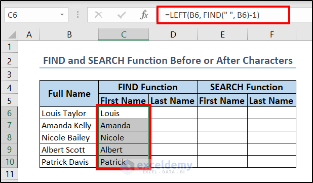
- FIND(” “, B6) searches for an empty string in the value of cell B6. In this case, it returns 6.
- LEFT(B6, FIND(” “, B6)-1) then extracts the first 5 characters from the left of the string. This is the word that comes before the empty space and thus the first name. 1 was extracted in the formula as it would take the space too otherwise.
-
- Now fill the range D6:D10 with the following formula.
=RIGHT(B6,LEN(B6)-FIND(" ",B6))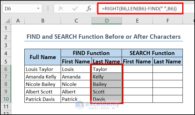
- LEN(B6) returns the length of the character in cell B6. In this case, it is 12.
- FIND(“ ”,B6) searches for the first empty string in cell B6, which is 6.
- LEN(B6)-FIND(” “,B6) gives the number of characters after the space in the string. In this case, it is 6.
- RIGHT(B6,LEN(B6)-FIND(” “,B6)) extracts the final 6 characters from the string and gives us the last name.
- Now insert the value in cell E6 and replicate it to E10.
=LEFT(B6, SEARCH(" ", B6)-1)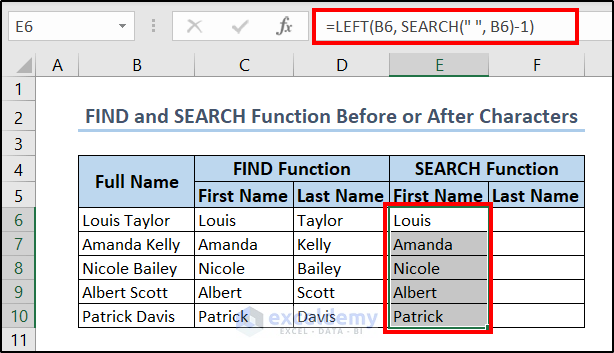
- SEARCH(” “, B6) searches for the space in cell B6, which is 6 in this case.
- LEFT(B6, SEARCH(” “, B6)-1) returns a number less than the previous function returns as we don’t want the space to include it in the first name.
- Using the following formula for the range F6:F10 will result as follows.
=RIGHT(B6,LEN(B6)-SEARCH(" ",B6))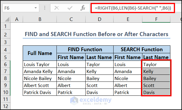
- LEN(B6) returns the length of the characters in cell B6.
- SEARCH(” “,B6) searches for an empty string in cell B6 and returns the first one it finds from left to right.
- LEN(B6)-SEARCH(” “,B6) indicates the characters available after the space in cell B6.
- RIGHT(B6,LEN(B6)-SEARCH(” “,B6)) then extracts the characters from the right of the string which is the last name from cell B6.
As we can see from four different formulas from the full list of names, there are no differences in the results. The reason behind this is there is no case difference while searching for an empty string. So we can use FIND and SEARCH functions interchangeably in these cases.
2. Merging with MID Function to Find String Between Parentheses
Like space as the string argument, we can both FIND and SEARCH functions for parenthesis too. Take the following dataset containing different product IDs.
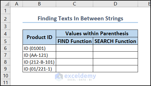
- Select cell C6, insert the following formula and replicate it to the end of the column.
=MID(B6,FIND("(",B6)+1, FIND(")",B6)-FIND("(",B6)-1)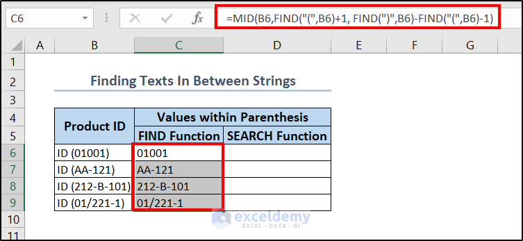
- FIND(“(“,B6) searches for the position of the opening parenthesis in cell B6, which is 4 here.
- FIND(“)”,B6) searches for the closing parenthesis which is at the 10th position. So it returns 10.
- FIND(“)”,B6)-FIND(“(“,B6)-1 is one less than the difference between closing and opening brackets. The significance of it is it indicates the number of characters in between the brackets. In this case, it is 5.
- MID(B6,FIND(“(“,B6)+1, FIND(“)”,B6)-FIND(“(“,B6)-1) extracts 5 characters from the string, starting from the 5th position(+1 in the starting argument). In the end, we get what is between the brackets in this way.
- To do the same with the SEARCH function, insert the following formula in cell D6 and replicate it till the end of the column.
=MID(B6,SEARCH("(",B6)+1, SEARCH(")",B6)-SEARCH("(",B6)-1)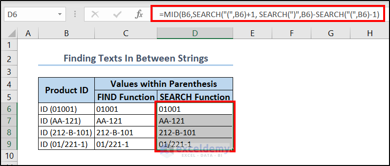
- SEARCH(“(“,B6) searches for the opening parenthesis of the value of cell B6 which is 4 in this case.
- SEARCH(“)”,B6) searches for the closing bracket in the value of cell B6 which is 10.
- SEARCH(“)”,B6)-SEARCH(“(“,B6)-1 is one less than that of the position of closing and opening brackets. The -1 at the end is there because the simple difference would include the closing bracket too.
- MID(B6,SEARCH(“(“,B6)+1, SEARCH(“)”,B6)-SEARCH(“(“,B6)-1) then extracts all the characters starting from the 5th position to the 9th which is the string inside the parentheses.
As we can see the outputs are the same in both of the cases. This is because there are no case differences in the opening or closing brackets. There is no wildcard usage here either. So, no matter the function we are combining it with, it gives the same result.
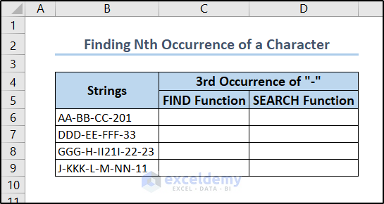
3. FIND and SEARCH Function to Find Nth Occurrence of Character
We can do the same for all the special characters and lowercase alphabetic characters. In this section, we will discuss the usage of FIND and SEARCH function in Excel. Much like the previous examples, it should end up with the same result too unless at least an uppercase value is involved.
We are going to operate with the following dataset for this example. The dataset contains a set of strings with a hyphen (-) between them. We are going to find the position of the 3rd hyphen in the string with both the FIND and SEARCH functions.
- First, enter the following formula in cell C6 and copy it down to cell C9.
=FIND("-",B6, FIND("-", B6, FIND("-",B6)+1) +2)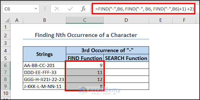
- FIND(“-“,B6) searches for a hyphen in the string of cell B6, which it finds at the third position.
- FIND(“-“, B6, FIND(“-“,B6)+1) Here the third argument is the optional argument that indicates the main FIND function to start the search from here. FIND(“-“,B6) actually is the first hyphen as mentioned earlier. So using it alone gives the second hyphen position.
- Now using the previous formula as the argument of the main function, it will start the search from the second hyphen. As a result, the final output will be the position of the third hyphen.
- Then in cell D6, we are going to use the following formula.
=SEARCH("-",B6, SEARCH("-", B6, SEARCH("-",B6)+1) +2)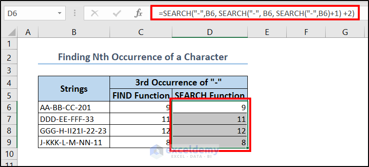
- SEARCH(“-“,B6) searches for the hyphen in the string of cell B6, which it finds at the third position.
- SEARCH(“-“, B6, SEARCH(“-“,B6)+1) The third argument is the optional argument that indicates the main SEARCH function to start the search from here. SEARCH(“-“,B6) actually is the first hyphen as mentioned earlier. So using it alone gives the second hyphen position.
- Now using the previous formula as the argument of the main function, it will start the search from the second hyphen. As a result, the final output will be the position of the third hyphen.
Even looping the FIND and SEARCH function with themselves give the same output as long as the string it search for is the same and case insensitive.
4. Error Handling with FIND and SEARCH Function in Excel
The FIND and SEARCH function returns an error while not encountering the values they search for. We can combine them with the IFERROR function. This will allow the spreadsheet to not show the error values. Instead, it will give us the output we want in those cases.
As long as the arguments are case insensitive and wildcards are not used, the function will give us the same values.
The following dataset contains some quotes in column B. We are going to search where “great”s are inside these quotes.

- For the range C6:C10, we are going to use the following formula to replicate.
=IFERROR(FIND("great",B6), "value not found!")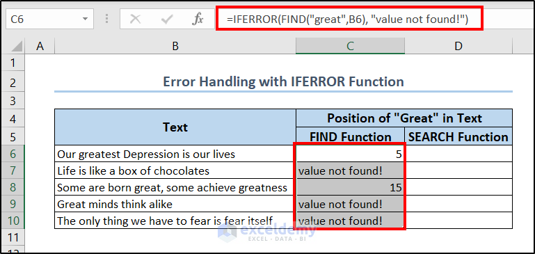
- FIND(“great”,B6) searches for the string “great” in cell B6 and returns the position of “g” in the first match from left to right.
- If there are no matches of the string in the desired cell, IFERROR(FIND(“great”,B6), “value not found!”) returns another string “value not found!”
- In the range D6:D10, we are going to use the following formula.
=IFERROR(SEARCH("great",B6), "value not found!")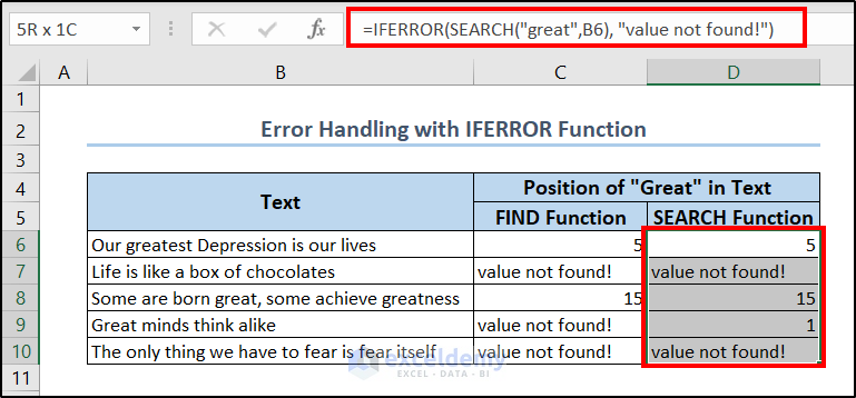
- SEARCH(“great”,B6) searches for the string “great” in cell B6. It also returns the first position of the character the first place it finds the match from left to right.
- IFERROR(SEARCH(“great”,B6), “value not found!”) returns another string “value not found!” if the SEARCH function doesn’t find any match for the value.
Notice that we have used a case-sensitive search here. The quote in cell B9 is an uppercase “Great”. So, the FIND function encounters an error here and gives a different result than the SEARCH function. Other values are the same. Because if the string “great” exists in them they are in the lower case.
So, as long as the upper/lower case in the string is not of concern, the FIND and SEARCH function gives the same output no matter how we use them.
Causes of #VALUE! Error in FIND and SEARCH Function in Excel
We have already seen a #VALUE! error in the wildcard example. It happened there because the FIND function couldn’t find an exact match in the string. There are other causes of the #VALUE! Error for FIND and SEARCH function in Excel.
- If there are any invalid arguments in the functions such as number or text values, it results in a #VALUE!
- When the string which we are searching the particular string from, or the second argument is not Excel’s text type value, it causes the error.
- The circular references where the result of the function depends on its own result, the function gives us the #VALUE!
- If you use any array arguments and do not press Ctrl+Shift+Enter, it may cause the #VALUE!.
Frequently Asked Questions
- How do I search for Find and Select in Excel?
You can press Ctrl+G on your keyboard for the shortcut to launch the Find and Select feature. Or, you can find that in Home > Find & Select (available in the Editing group) > Go to.
- How do I find and select all values in Excel?
To select all cells with values in a dataset, select a cell within it and press Ctrl+A on your keyboard. If you select a blank cell instead, it will select all of the cells in the spreadsheet.
- How do I search and extract text in Excel?
You can extract text from a string using a combination of LEFT, RIGHT, MID, LEN, etc functions along with FIND or SEARCH functions. A little bit of it is shown in the similar uses section. For more details, you can check out this article- how to extract text from a cell in Excel.
Things to Remember
- Both functions use the same set of arguments- a string to look for, where it will look, and the starting point from where it will search.
- If you need to perform a case-sensitive search, use the FIND Otherwise, you use the SEARCH function.
- For wildcard uses definitely use the SEARCH function.
- For non-alphabetic character searches, you can search with either of the functions.
- Be sure to use the third argument in cases where you need to skip some of the first matches.
- Both functions only work with text values.
Download Practice Workbook
You can download the workbook used for the demonstration from the link below.
Conclusion
That concludes the discussion of similarities and differences between the FIND and SEARCH functions in Excel. The main thing to keep in mind for everyday usage is case sensitivity, even while combining with other functions. Hopefully, you can use both functions to find string positions and apply them to your formulas with ease now. I hope you found this guide helpful and informative. If you have any questions or suggestions, let us know in the comments below.
<< Go Back to Excel Functions | Learn Excel

