Name Box in Excel (All You Need to Know)

In this article, we will learn about the Name Box in Excel. We will focus on naming different kinds of elements, displaying the names in the Name Box, and many more in this article.

Name Box usually displays the names of selected worksheets or workbook elements. You can use the Name Box to make necessary edits or perform required operations on a cell or range of cells. The Name Box is handy, especially when working on a large dataset.

What Is a Name Box in Excel?

Name Box is a portion of an Excel worksheet where the name of an element (cell, range of cells, chart, etc.) appears. For example, if you select any cell of the worksheet, you will get the name of the cell in the Name Box.

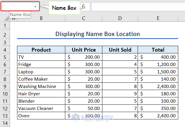
Name Box Location

• You’ll find the Name Box in the top left corner of the dataset, just on the left side of the formula bar.

How to Display Name of an Element in a Name Box in Excel

You can check the name of any element (cells, range of cells, chart, etc.) in the Name Box. We will review the details individually.

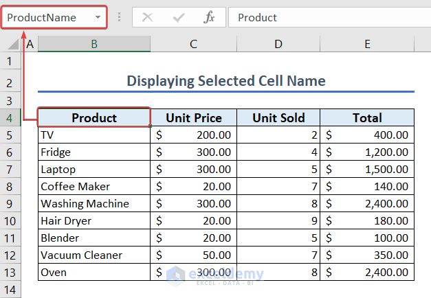
1. Displaying Selected Cell Name

• If you select any cell in the worksheet, the corresponding cell name will appear in the Name Box.
• Select cell B4.
• The name of cell B4 (ProductName) will appear in the Name Box.

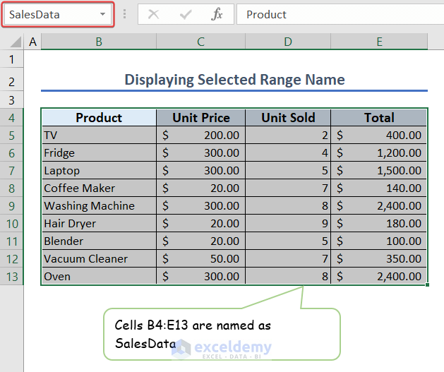
2. Displaying Selected Range Name

• The corresponding range name will appear in the Name Box if we select a range of cells in the worksheet.
• Select cells B4:E13.
• You will get the name of this range of cells SaleData in the Name Box.

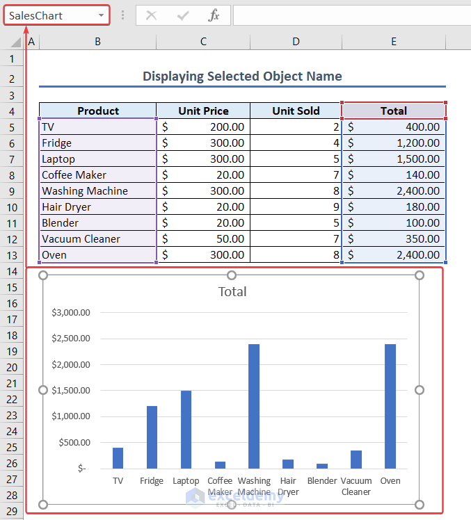
3. Displaying Selected Object Name

• If you select any object in the worksheet, the name will appear in the Name Box.
• Select the chart.
• In the Name Box, you’ll see the chart name (SalesChart).

How to Use a Name Box in Excel

We can use the Name Box for multiple purposes. We can navigate to a specific cell quickly, select a range of cells, and many more using the Name Box.

1. Navigating to a Specific Cell Quickly

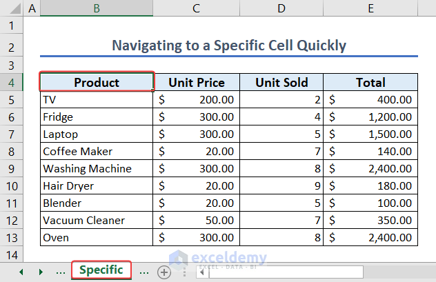
• You need to scroll a lot to navigate to a distant cell.
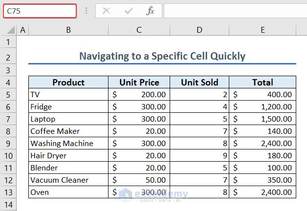
• Alternatively, you can type the cell address in the Name Box to navigate to the cell.

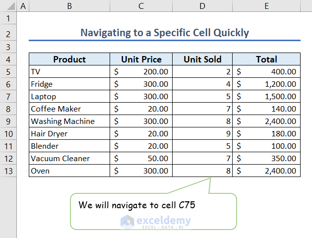
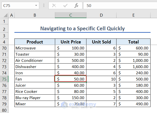
• Type C75 in the Name Box and press ENTER to navigate to cell C75.

• As a result, cell C75 will be activated.

2. Navigating to an Intersecting Range

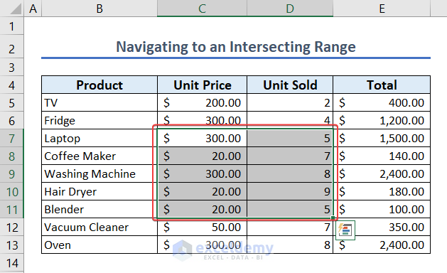
• If we type two ranges of cells in the Name Box and press ENTER, the intersection of the two ranges will be selected.
• Type B6:D11 C7:E12 in the Name Box and hit ENTER.

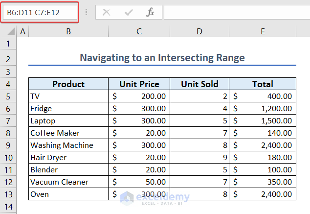
• As a result, the intersection of the two ranges is selected now.

3. Navigating to a Specific Worksheet

• If we type any worksheet’s name followed by a cell address, the mentioned cell in that worksheet will be selected.
• We have a worksheet named Specific and we want to select the B4 cell of that worksheet using the Name Box.

• Type Specific!B4 in the Name Box and hit ENTER.

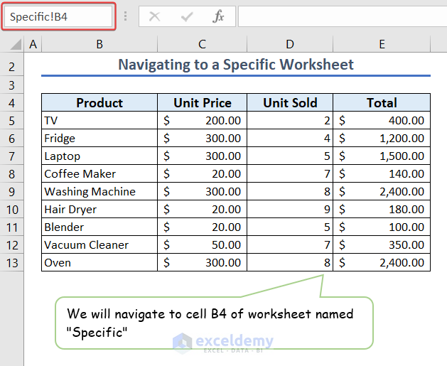
• As a result, cell B4 of the worksheet named Specific will be selected.

4. Navigating to a Specific Workbook

• We can also navigate to a different workbook by using the Name Box.
• We will navigate to cell B15 of the workbook named Shop2.

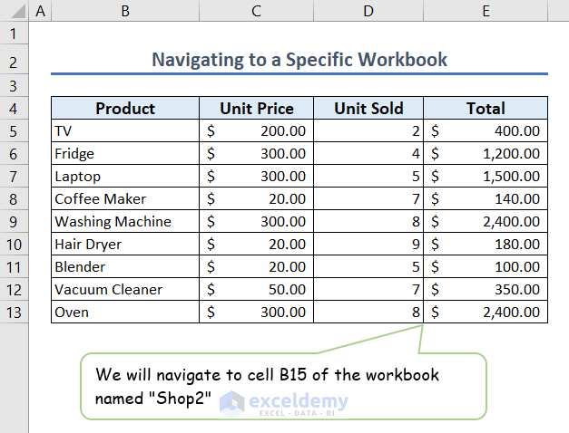
• Type [Shop2.xlsx]Shop2Total!B15 in the Name Box and hit ENTER.

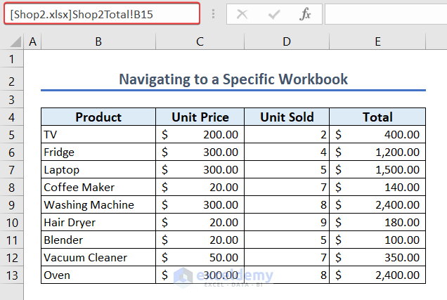
• As a result, we will be moved to the B15 cell of the workbook named Shop2.

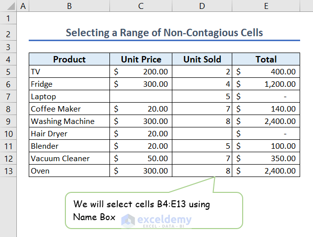
5. Selecting a Range of Non-Contiguous Cells

• You can select a range of non-contiguous cells using the Name Box.
• We will select cells B4:E13 using the Name Box.

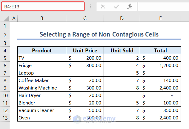
• Type B4:E13 in the Name Box and press ENTER.

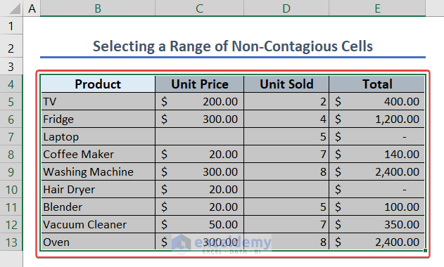
• Hence, cells B4:E13 will be selected.

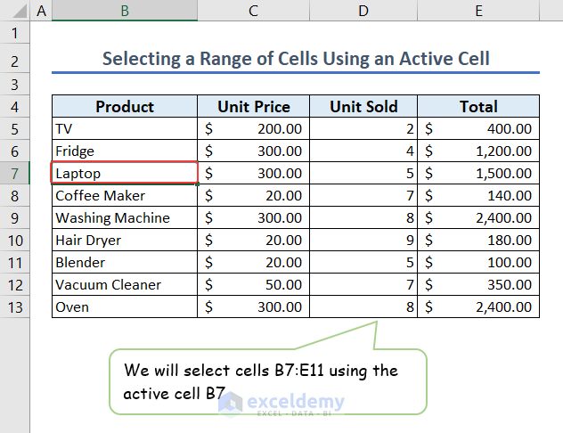
6. Selecting a Range of Cells Using an Active Cell

• You can select a range of cells by utilizing an active cell.
• B7 is the active cell in this case.
• We will select cells B7:E11 using the active cell B7.

• Type E11 in the Name Box and press Shift + ENTER.

• Consequently, cells B7:E11 will be activated.

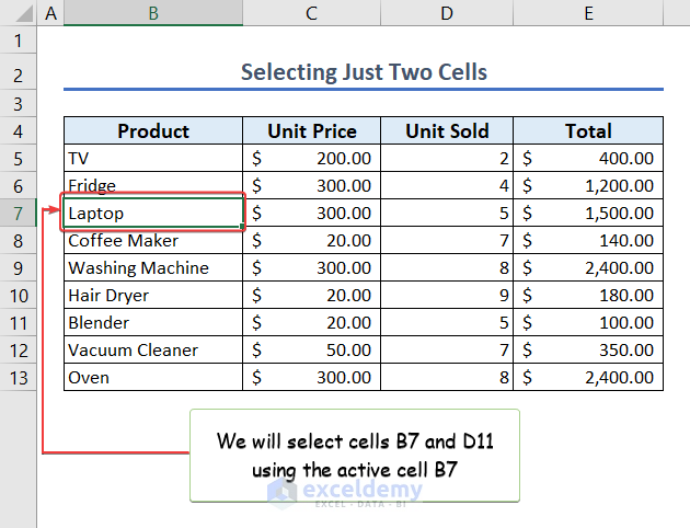
7. Selecting Just Two Cells

• We will select cells B7 and D11 using the active cell B7.

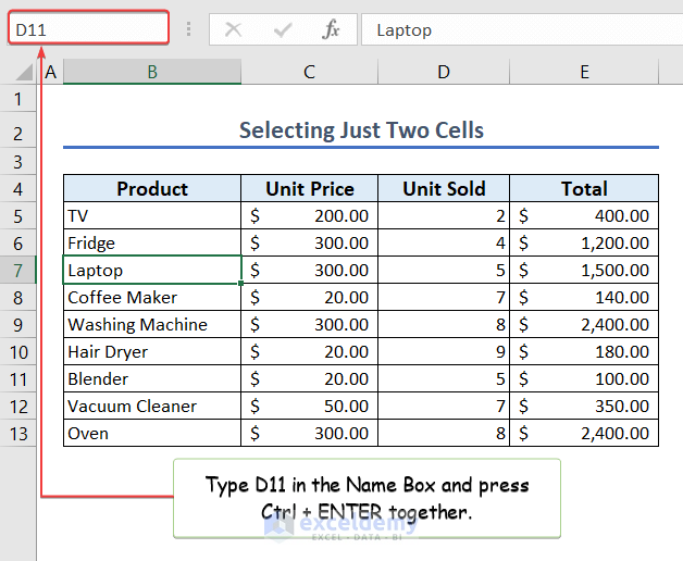
• Type D11 in the Name Box and press Ctrl + ENTER together.

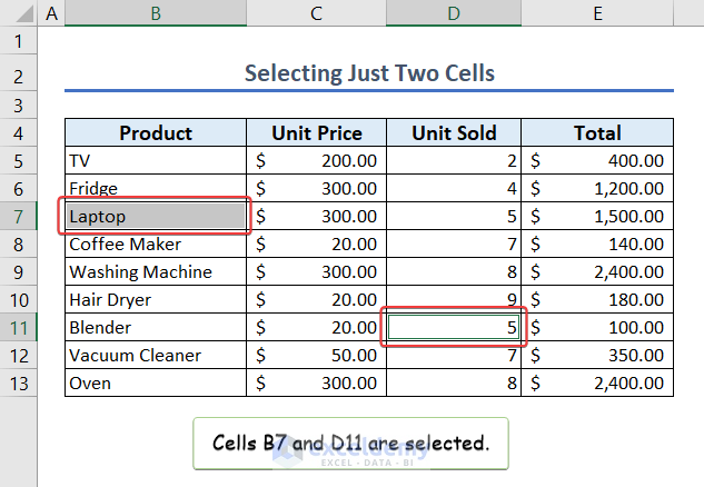
• In this way, cells B7 and D11 will be selected.

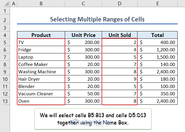
8. Selecting Multiple Ranges of Cells

• We will select cells B5:B13 and cells D5:D13 together using the Name Box.

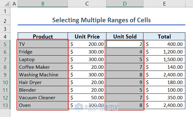
• Type B5:B13,D5:D13 in the Name Box and press ENTER.

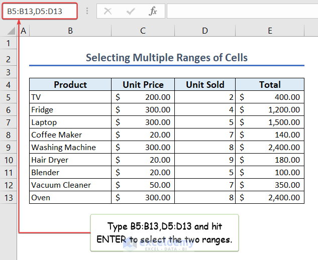
• As a result, the two ranges of cells will be selected.

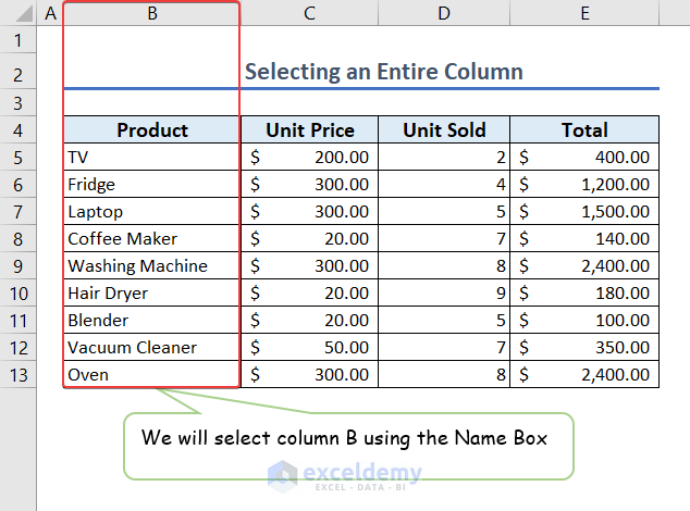
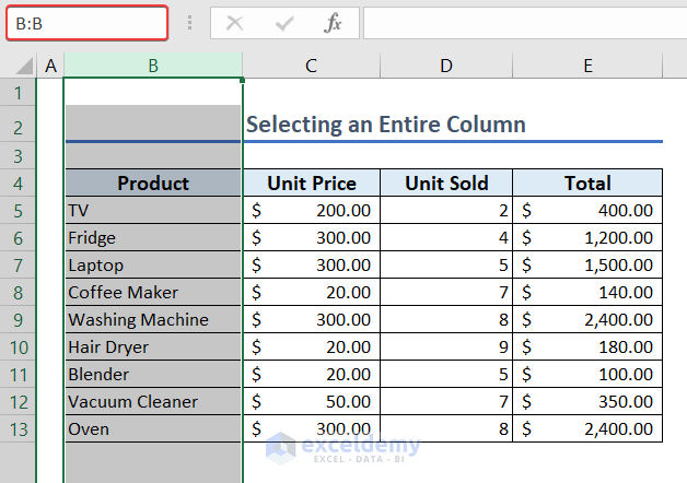
9. Selecting an Entire Column

• You can select an entire column using the Name Box.
• In this case, we will select column B.

• Type B:B in the Name Box and press ENTER.
• As a result, column B will be selected.

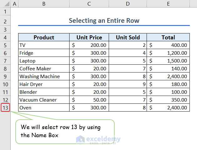
10. Selecting an Entire Row

• We will select row 13 by using the Name Box.

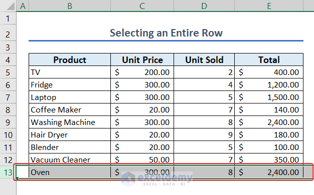
• Type 13:13 in the Name Box and hit ENTER.

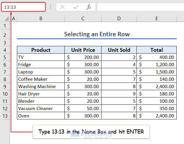
• In this way, row 13 will be selected.

11. Selecting Named Range from Name Box

• Here, we will use a different dataset.
• To select a Named Range from a Name Box, click on the arrow of the Name box.

• Select Students_marks named range from the drop-down menu.
• Thus, the dataset with this name will be selected.

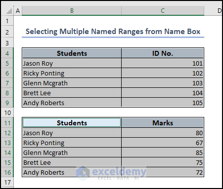
12. Selecting Multiple Named Ranges from Name Box

Here, we will show how you can select multiple named ranges from the Name box.

• Select the first named range >> the dataset of that named range will be selected.
• Then, press and hold the CTRL key >> select the second named range.

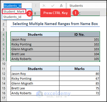
• Thus, you can select the second dataset as well.

13. Displaying Information about Cells

The Name Box displays information about a cell. It displays the cell address or row and column count depending on the selection method.

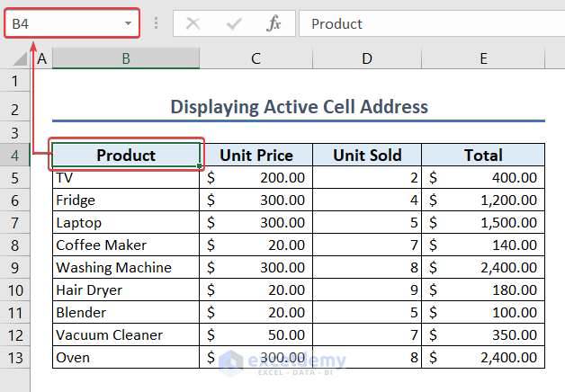
13.1 Displaying the Active Cell Address

• If we click on any cell of the worksheet, the corresponding cell address will pop up in the Name Box.
• Select the cell that contains the Product.
• And you’ll see B4 in the Name Box.

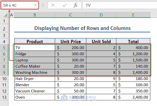
13.2 Displaying Number of Rows and Columns of a Selected Range

• If we hold the mouse or Shift key while selecting the cells in the worksheet, the Name Box will display the number of selected rows and columns.
• Select cells B5:E9.
• The Name Box will display the selected row and column count.

How to Use Name Box Drop-Down Option in Excel

We can use the drop-down icon of the Name Box in various ways.

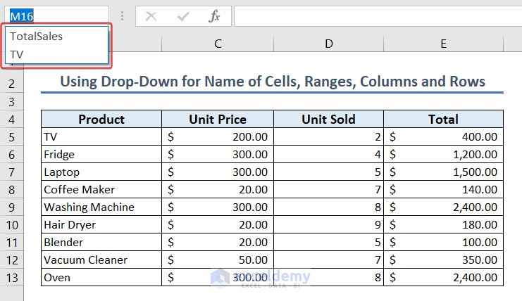
1. Using Drop-Down for Name of Cells, Ranges, Columns and Rows

• Select the drop-down icon of the Name Box.

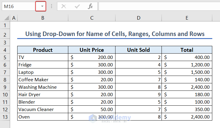
• The named elements will show up as a result.

2. Using Drop-Down for Recently Used Formulas

• You can use the Name Box to utilize the recently used formulas.
• Type = in cell E14.
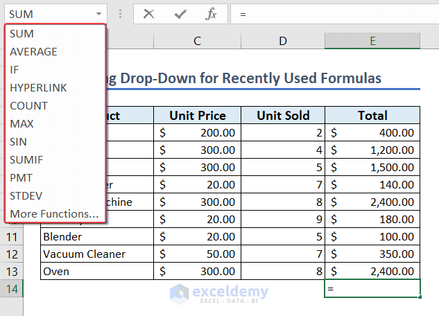
• Click on the drop-down icon of the Name Box.

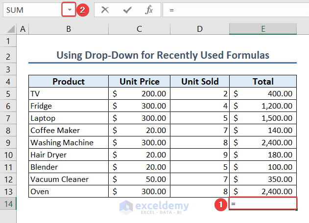
• As a result, you will get a list of recently used formulas.

How to Name a Range of Cells

• We will name the range of cells B5:B13 using the Name Box.

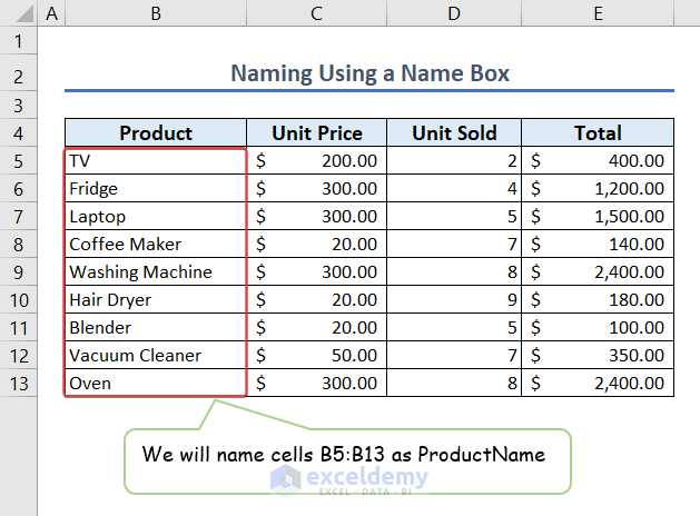
• Select cells B5:B13.
• Type ProductName in the Name Box.

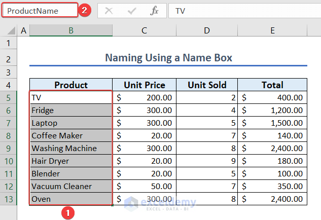
• As a result, cells B5:B13 are now named as ProductName.

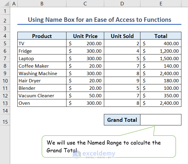
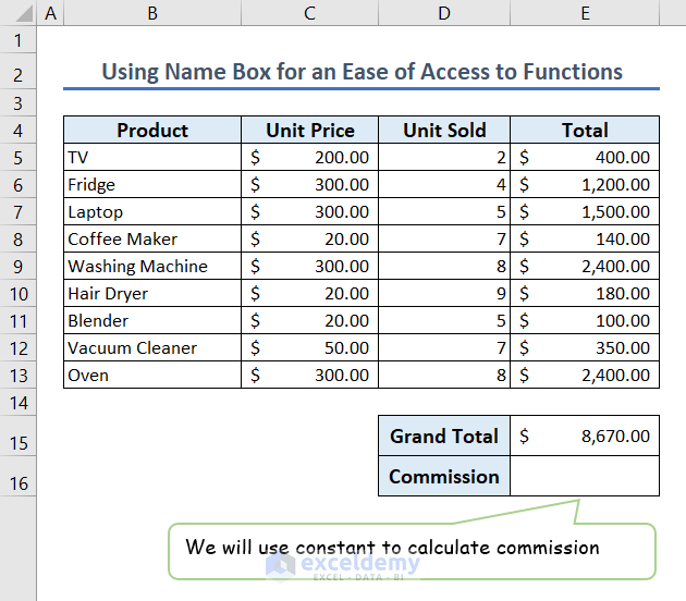
How to Use Name Box for an Ease of Access to Functions

• You can use a named range as an argument of a function.
• We’ve named cells E5:E13 as SalesTotal.
• We will use this name to calculate the grand total.

• Type the following formula in cell E15 and press ENTER.

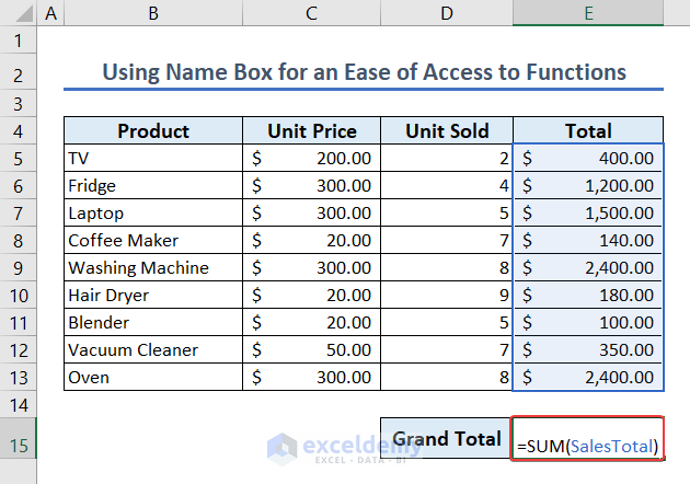
• As a result, we will get the grand total.

• You can create a constant using the Name Manager.
• We will set the commission rate as constant and use it later to calculate the commission.

• Navigate to Formula >> Name Manager.

• Click on New.

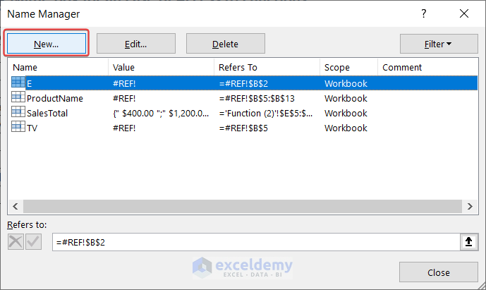
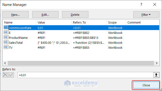
• Type the following information as shown in the image below and click OK.

• In this way, commissionRate constant is set.

• Type the following formula in cell E16 and hit ENTER to calculate the commission.

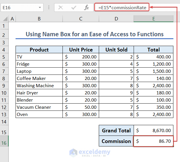
Edit or Delete a Named Range in Excel

• You can either edit or even delete a name using the Name Manager.
• Go to Formulas >> Name Manager.

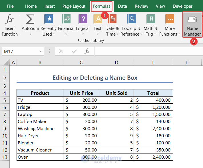
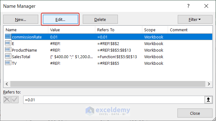
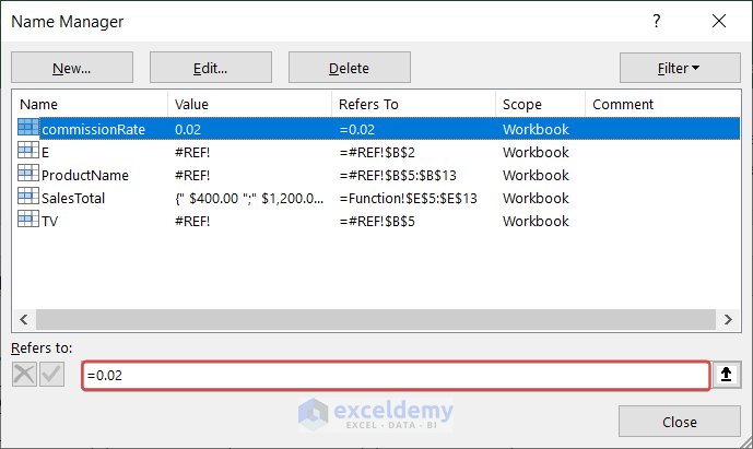
• Select Edit to edit the name commissionRate.

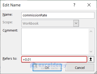
• You can edit any field according to your need.
• commissionRate initially refers to a value of 0.01.
• We will edit this value.

• Edit the value as 0.02 and click OK.

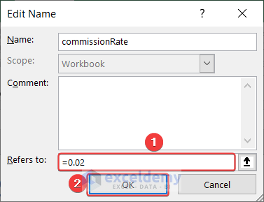
• As a result, Excel will edit the value.

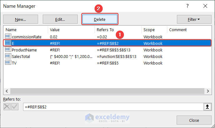
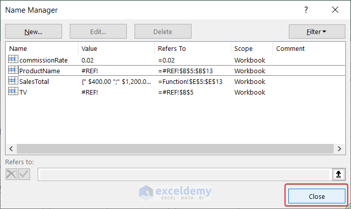
• If you want to delete any name, you can do that too.
• Select the name E.
• Click on Delete to delete the name.

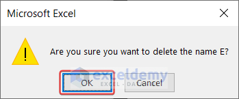
• A warning message will pop up.
• Click OK.

• As a result, Excel will delete the named ranges.

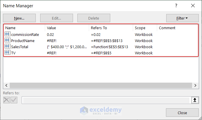
• Finally, click on Close to close the name manager window.

Things to Remember

While working with Name Box in Excel, remember the following facts.

• If you want to select only a single column or row using the Name Box, ensure that that particular column or row is not part of a merged column or row.
• Double-check before deleting any name using the Name Manager, which may create a reference error.
• Avoid using punctuation while naming any element.

Download Practice Workbook

You can download the workbook from here and practice yourself.

Conclusion

We have demonstrated the details of the Name Box in Excel in this article. If you have followed this article carefully, now you can apply names to the Excel elements, edit or delete the name, and so on- all by yourself. If you face any problem doing so, please let us know in the comment section. Team Exceldemy will be happy to help you out regarding the problems. Have a good day.

Frequently Asked Questions

1. How do I Open a Name Manager in Excel?

You can navigate to Formulas >> Name Manager to open a Name Manager in Excel.

2. What is the shortcut key for Name Box in Excel?

Alt + F3 is the shortcut key for the Name Box in Excel.

3. What is a label in Excel?

The text we type in a cell is the label in Excel.

Name Box in Excel: Knowledge Hub

• How to Name a Cell in Excel
• How to Edit Name Box in Excel

<< Go Back to Excel Parts | Learn Excel