In Microsoft Excel, there are several methods to name a range and make it also dynamic simultaneously. The named ranges are easy to prepare. They are fun to use since they store an array of strings that we don’t need to specify with cell references manually. In this article, you’ll get to know all possible and suitable methods to name a range in Excel with examples and simple explanations.
Download Practice Workbook
You can download the Excel workbook that we’ve used to prepare this article.
What Is a Named Range in Excel?
A named range is a range of cells or an array that is assigned with a user-defined name. A named range can be used in a function or a formula instead of selecting the corresponding range of cells manually.
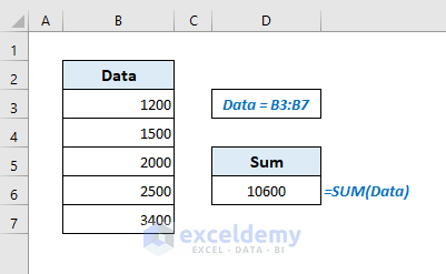
The following is an example of using a named range. The range of cells, B3:B7 has been named with Data. In the output Cell D6, we’ve performed a simple sum of all values present in that named range. We could’ve typed the formula with “=SUM(B3:B7)”, but we have used the named range Data instead here. While dealing with large formulas, the named range is a handy operator there to input the specific range of cells with ease.
Benefits of Using a Named Range in Excel
Let’s go through the following points that might persuade us to use a named range frequently in Excel spreadsheets.
- While using the named range in a formula or function, we can avoid using cell references.
- Due to the use of a named range, we don’t have to go back to our dataset every time while entering a range of cells.
- Once created, the named range can be used in any of the worksheets in a workbook. The named range is not limited to use in a single worksheet only.
- The named range makes a formula dynamic which means if we define a formula with a name, we can also use that named range to perform calculative operations instead of typing a combined and huge formula.
- Excel allows a named range to be dynamic with additional inputs from the user.
Read More: How to Use Named Range in Excel VBA (2 Ways)
Some Rules to Name a Range of Excel Cells
There are some conventions for naming a range of cells. We can have a glance at those rules to keep them in memory while defining names for the selected ranges.
- No space character is allowed to use in the name of a range.
- The names cannot be with the cell addresses (e.g: C1, R1C1).
- You cannot name a range with only ‘R’ or ‘C’. These are the indicators of rows and columns in Excel.
- Names are case-insensitive. It means both ‘Sales’ and ‘SALES’ will work as the similar named range of cells.
- The name of a range cannot exceed 255 characters.
- Except for backlash (\) or underscore (_), almost no other punctuation mark is allowed to use while naming a range of cells.
5 Quick Approaches to Name a Range in Excel
1. Use ‘Define Name’ Command to Name a Range
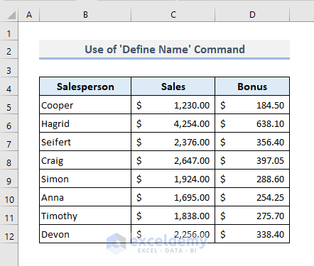
Now we’ll see some of the examples where we’ll learn how to name a range of cells easily in an Excel spreadsheet. The dataset in the following picture represents several random names of salespersons, their sales amounts, and a bonus amount of 15% for their corresponding sales.
Let’s say, we want to name the range of cells, C5 to C12 with ‘Sales’. And in our first method, we’ll apply the Define Name command from the Excel ribbon options.
📌 Step 1:
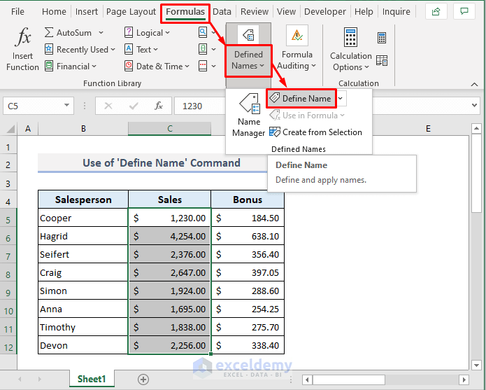
➤ First, select the range of cells, C5 to C12.
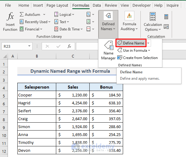
➤ Under the Formulas tab, select the option Define Name from the Defined Names drop-down. A dialog box will appear.
📌 Step 2:
➤ Type ‘Sales’ in the Name Box or you can input any other name you want. As we’ve selected the range of cells (C5:C12) before, they’ll be visible in the Refers to box.
➤ Press OK and your named range is now ready to use.

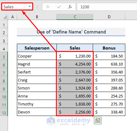
Now if we select the range of cells C5 to C12, we’ll find the newly created name of that range in the Name Box at the left top corner as shown in the image below.
We can now use that named range anywhere in our worksheets. We have to simply insert an equal sign (=) in a cell and type the created name of a range of cells.
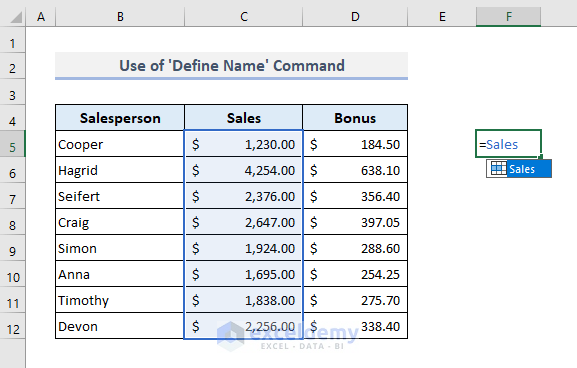
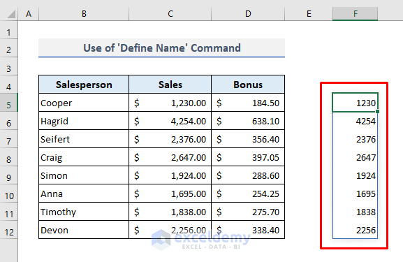
And after pressing Enter, the named range will return an array including all the values that are present within the range of cells: C5 to C12.
Read More: How to Edit Defined Names in Excel (Step-by-Step Guideline)
2. Name a Range of Cells by Using ‘Name Manager’
We can also use the Name Manager feature from the Formulas ribbon. It will allow you to view or customize a named range with multiple options. The steps are simple as follows:
📌 Step 1:
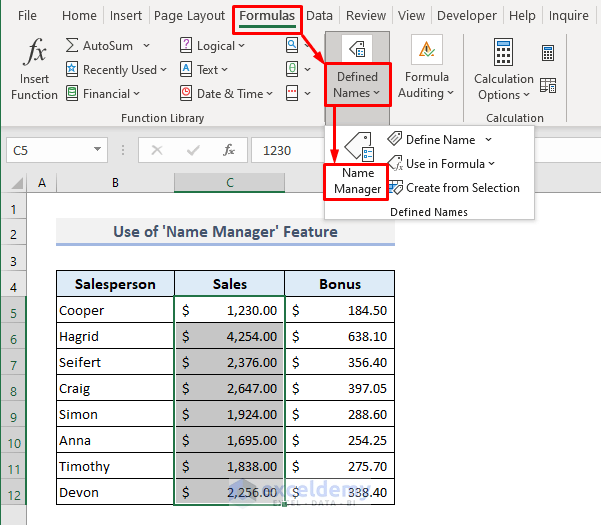
➤ Select the data range that you want to give a specific name.
➤ Under the Formulas tab, choose the option Name Manager from the Defined Names drop-down. A dialog box will open up.
📌 Step 2:
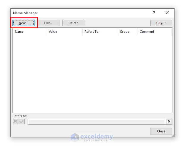
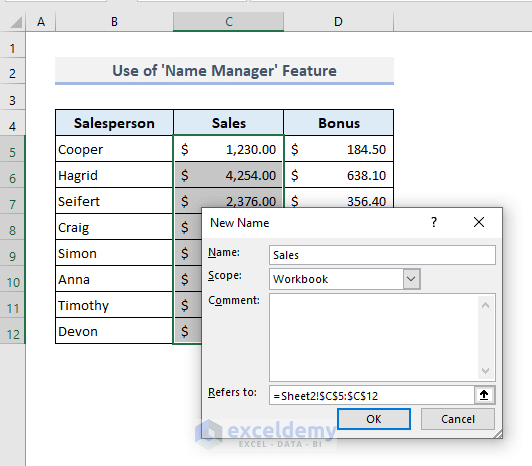
➤ Click on the New tab.
📌 Step 3:
Now the procedures are similar as shown in the first method to define a name of the selected range of cells. So, refer to your data range and give it a specific name in the particular boxes.
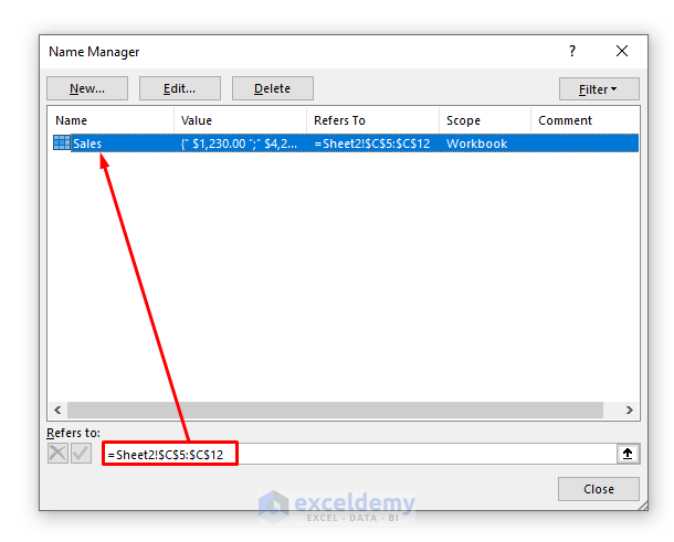
The Name Manager window will reappear now where you’ll find the newly given name of your cell ranges.
📌 Step 4:
➤ Press Close and you’re done.
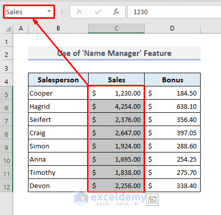
Now if you select your data range in the Excel worksheet, you’ll see the name assigned for it in the Name Box.
Read More: How to Edit Name Box in Excel (Edit, Change Range and Delete)
3. Apply ‘Create from Selection’ Tool to Name an Excel Range
By utilizing the previous two methods, you can select the reference cells before or after selecting the tools from the Excel ribbons. Now if you don’t want to name a range of cells manually, then this method is suitable for you. Here, you have to select a data range along with its header and the Create from Selection tool will define a name for the range by detecting its header.
This method is actually time-saving and quite flexible to name a range of cells in an Excel spreadsheet. The necessary steps are as follows:
📌 Step 1:
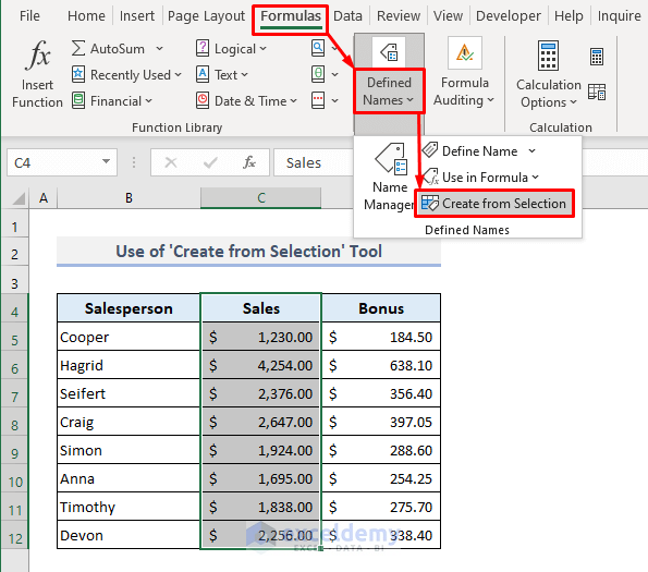
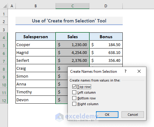
➤ Select the range of cells (C4:C12) that you want to name along with its header. In our dataset, Cell C4 contains the header which we’ll use as the name for our data range (C5:C12).
➤ Under the Formulas tab, choose the Create from Selection command from the Defined Names group of commands or drop-down. A dialog box will appear.
📌 Step 2:
➤ Mark on the first option ‘Top Row’ as our header name is at the top of the selected column.
➤ Press OK and we have just created our named range!
Now we can select our data range and find the name of the selected range in the Name Box.

Read More: Excel VBA to Create Named Range from Selection (5 Examples)
4. Edit ‘Name Box’ to Name a Range in Excel
Using a Name Box to specify a range of cells with a name is quite easier than all previous methods. But a problem with using this method is you cannot edit a name anymore or even you won’t be able to delete the name once you have created it. So afterward, you have to launch the Name Manager to edit or delete the specified named range.
We can use the Name Box to define the selected range of cells with a name only.
📌 Steps:
➤ First, Select the range of cells to be defined with a specific name.
➤ Now, go to the Name Box and type a name for the selected range.
➤ Finally, press Enter and you’re done.
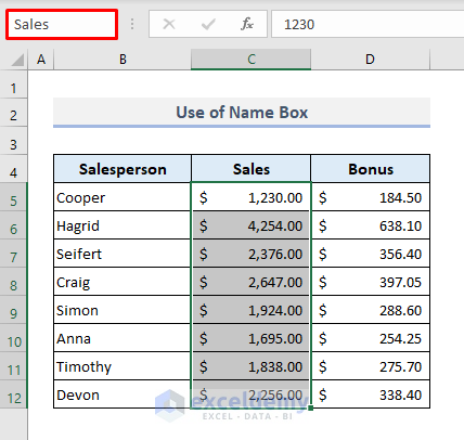
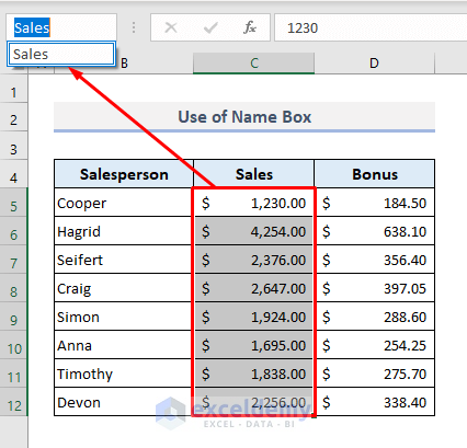
Now open the drop-down list in the Name Box and you’ll find the newly created name there for the selected range of cells.
Read More: [Fixed!] Name Manager Delete Option Greyed out in Excel (3 Reasons)
5. Create a Dynamic Named Range in Excel
In all methods described so far, we’ve named a range for a fixed range of cells. Now let’s say, we want to name a range that is not static, which means we can input more data that will create a dynamic range of cells. And the named range will be expanding based on our data inputs.
For example, we’ve named a range of cells (C5:C12) in Column C. But now we have to input more data from the bottom of Cell C12. But if our named range is not set to dynamic, the additional inputs will not be counted for the named range once defined.
So, to make our named range dynamic, we have two interesting options. We can use an Excel table or we can use a formula with the OFFSET function. Now we’ll find out how both of the methods work out in the following sections.
5.1 Using an Excel Table
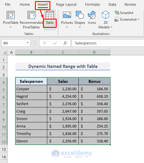
First of all, we’ll insert an Excel table to make our range of cells dynamic. In our dataset, we have headers in Row 4 for the table range containing cells starting from B4 to D12.
📌 Step 1:
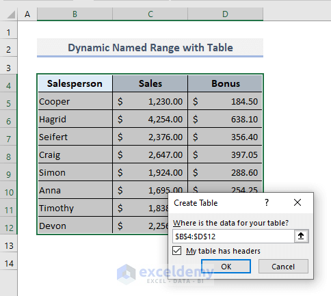
➤ Select the range of cells (B4:D12) first.
➤ From the Insert ribbon, choose the Table option.
📌 Step 2:
➤ In the Create Table dialog box, press OK only as all the parameters are set automatically which we don’t need to alter right now.
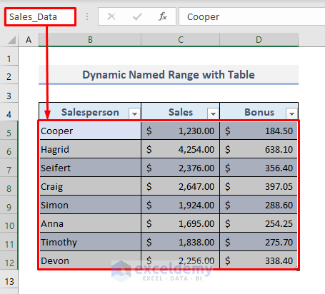
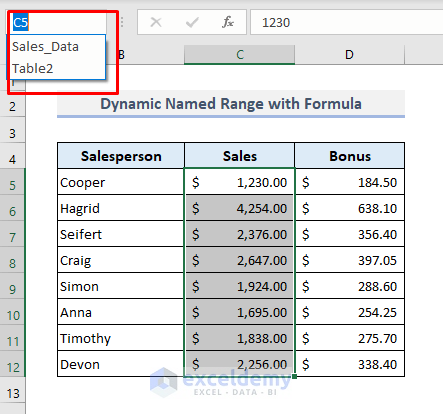
As shown in the picture below, our data range has now turned into a table. The default name of this newly created table usually becomes Table1 if no other table has not been formed in that workbook before. In the Name Box, we can rename this range of data with something else according to our preference. Let’s say, we have defined the table with the name, Sales_Data.
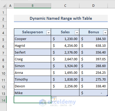
Now we’ll find out what will happen if we input any value in Cell B13 under the table range. We’ve entered a random name ‘Mike’ in Cell B13.

After pressing Enter, we’ll find that the table has expanded to the bottom row immediately.
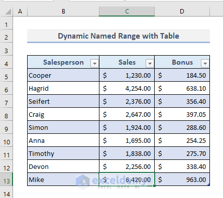
Since all the cells in the Bonus column are assigned with 15% of the sales amounts, now we’ll find out if it really works with additional input in Cell C13.
So, if we enter a sales amount (6420) in Cell C13, the bonus amount in Cell D13 will be displayed at once. It means our table range has expanded with its defined format and formulas.
If we want to be more certain of the expanded table range, then we can enable editing Cell D13. And we’ll see the assigned formula there which we have used previously for the rest of the cells in the Bonus column.

We can also input more data afterward from the bottom of the table and the defined table range will be expanding accordingly.

Read More: How to Set Value to a Named Range with Excel VBA (3 Methods)
5.2 Combining OFFSET and COUNTA Functions
The first method with the Table is quite easy to prepare a dynamic named range. But we can also use a formula combining the OFFSET and COUNTA functions to make a named range for our dataset. The OFFSET function returns a reference to a range that is a given number of rows and columns from a given reference. And the COUNTA function counts all the non-blank cells in a range. Now let’s see how we can use these functions together to make a dynamic named range in the following steps.
📌 Step 1:
➤ Under the Formulas tab, select the Define Name command from the Defined Names drop-down. A dialog box will open up.
📌 Step 2:
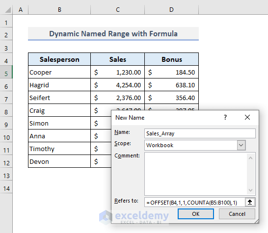
➤ Let’s say, we want to expand our named range up to 100 cells vertically. So, the required formula in the Reference box will be:
=OFFSET(B4,1,1,COUNTA(B5:B100),1)➤ Define this range of cells with a name, Sales_Array.
➤ Press OK and our dynamic named range is now ready for further uses.
But with this method, the name of the dynamic range will not be visible in the Name Box.
Again we can use this named range by pressing Equal (=) in any cell and typing the name of that defined range.
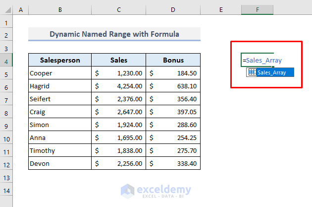
And after pressing Enter, the return array will look like the following. As we have made a named range for all sales data, so those values will appear only but no pre-specified format will exist in the array. Later we can format those return data manually if we need.

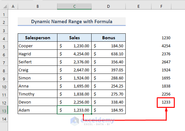
To make sure of the newly created dynamic named range, we can insert the specific values in an additional row (13). Since we have input a sales amount of 1233 in Cell C13, it’ll be added to the named range array immediately displayed on the right in the screenshot below.
Read More: How to Use Dynamic Named Range in an Excel Chart (A Complete Guide)
Edit or Delete a Named Range after Creation
After creating a named range, we may need to edit or even delete the named range. And to perform this, we have to open the Name Manager from the Formulas ribbon. Let’s see how to edit a named range first in the steps below. We’ll replace the name ‘Sales_Array’ with ‘Bonus_Amount’ here and the new range of cells will include all data from the Bonus column.
📌 Step 1:
➤ Launch the Name Manager window first from the Formulas tab.
➤ Click on the row containing data for Sales_Array.
➤ Push the Edit option. The dialog box called Edit Name will appear.

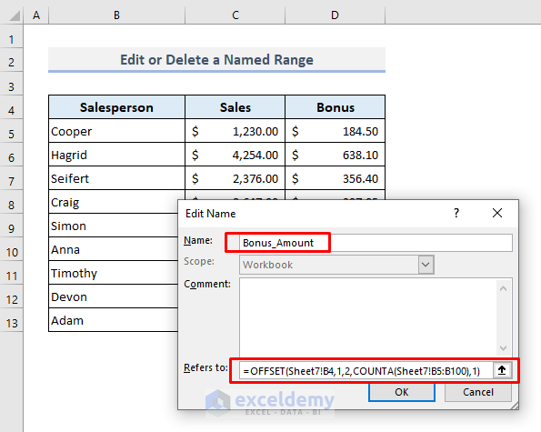
📌 Step 2:
➤ Enter a new name Bonus_Amount in the Name box.
➤ Type the following formula in the Reference box:
=OFFSET(Sheet7!B4,1,2,COUNTA(Sheet7!B5:B100),1)➤ Press OK.
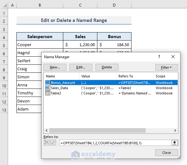
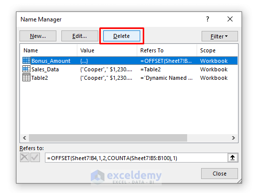
The Name Manager window will reappear itself where you’ll find the newly edited name range as displayed in the following image.
Now return to your worksheet and enable editing in any cell. Press the Equal (=) sign and type the edited name of the newly selected range.
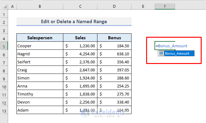
Press Enter and the bonus amounts will be shown in an array right away.

And finally, if you want to delete a named range, then simply select the corresponding row from the Name Manager and press the Delete button. The data range along with its specified name will be removed from the Name Manager.
Read More: How to Delete All Named Ranges in Excel (2 Ways)
Concluding Words
I hope all of the methods mentioned in this article will now help you to apply them in your Excel spreadsheets when you need to name a range only or even make it dynamic later. If you have any questions or feedback, please let me know in the comment section. Or you can check out our other articles related to Excel functions on this website.
Related Articles
- How to Delete Named Range in Excel (3 Methods)
- [Solved!] Names Not in Name Manager in Excel (2 Solutions)
- How to Change Excel Column Name from Number to Alphabet (2 Ways)
- Change Scope of Named Range in Excel (3 Methods)
- How to Name a Column in Excel (3 Easy and Effective Ways)
- Paste Range Names in Excel (7 Ways)

