If you are looking for some special tricks to know how to use OFFSET for cell reference in Excel, you’ve come to the right place. We’ll show 5 suitable methods to use OFFSET for cell reference in Excel. This article will discuss every step of the methods. Let’s follow the complete guide to learn all of this.
How to Use OFFSET for Cell Reference in Excel: 5 Easy Ways
The OFFSET function returns a reference to a range that is a given number of rows & columns from a given reference. This function begins with a cell reference, moves down a specified number of rows, then right a specified number of columns, and extracts a section. As a result, it returns data with a specific height and width, situated at a specific row down and column right from a specified cell reference. If the rows argument is negative, the function will move the specified number of rows upward.
Our Excel dataset will be introduced to give you a better idea of what we’re trying to accomplish in this article. We have a sales record of 5 months for 13 products of a company named ABC Company.
This section provides extensive details on these methods. You should learn and apply these to improve your thinking capability and Excel knowledge. We use the Microsoft Office 365 version here, but you can utilize any other version according to your preference.
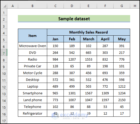
1. Extract Whole Row
Here, we will demonstrate how to extract a whole row from a dataset in Excel. We will try to sort out a whole row using the OFFSET function. Let’s try to extract the sales record for laptops for all the months.
📌 Steps:
- First, type the following formula to extract the sales records for laptops for all the months.
=OFFSET(B5,7,0,1,6)
The OFFSET function starts moving from cell B5. Then it moves 7 rows downward to find the laptop. And then it extracts out a section of 1 row height and 6 columns of width. This is the sales record of laptops from Jan to May.
- Then, press Enter.
- Consequently, the output will look like this.
Read More: How to Reference a Cell from a Different Worksheet in Excel
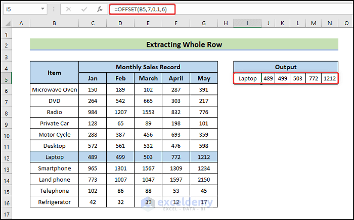
2. Extract Entire Column
Now we’ll sort out a whole column from the same set of data. Let’s try to find out all the sales in March. And we will extract a list of a total of 13 products. Let’s walk through the following process to sort out a whole column from the dataset.
📌 Steps:
- First, type the following formula to sort out a whole column from the dataset.
=OFFSET(B5,0,3,12,1)
The function starts moving from cell B5. It moves 1 row down. Then move 3 columns right to the month of March. Then it extracts a section of 12 rows in height (all the products) and 1 column width (only for the month of March).
- Then, press Enter.
- Therefore, the output will look like this.
Read More: How to Reference Cell in Another Sheet Dynamically in Excel
3. Obtain Adjacent Multiple Rows and Columns
The purpose of this section is to collect a section of the data set containing multiple rows and multiple columns. In January and February, let’s gather sales data on the products Motorcycle, Desktop, and Laptop. Following is a step-by-step guide to sorting out adjacent multiple rows and columns.
📌 Steps:
- First, type the following formula to sort out adjacent multiple rows and columns from the dataset.
=OFFSET(B5,5,0,3,3)
The function starts moving from cell B5. Then it moves 5 rows down to the product telephone. Then collects the data of 3 rows height.
- Then, press Enter.
- Therefore, the output will look like this.

Read More: How to Use Cell Value as Worksheet Name in Formula Reference in Excel
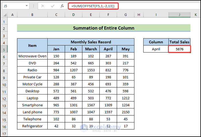
4. Get Summation of Entire Column
Here, we will demonstrate how to get the summation of an entire column by combining SUM and OFFSET functions in Excel. Let’s walk through the following steps to get the summation of an entire column.
📌 Steps:
- First, type the following formula in cell J5.
=SUM(OFFSET(F5,1,-2,13))
- Then, press Enter.
- Consequently, the output will look like this.
🔎 How Does the Formula Work?
- OFFSET(F5,1,-2,13)
The OFFSET function starts moving from cell F5. Then it moves 1 row downward and extracts the records of sales in the April column.
- SUM(OFFSET(F5,1,-2,13))
The OFFSET function’s output will be summed by the SUM function.
Read More: How to Find and Replace Cell Reference in Excel Formula
5. Find Average of Whole Column
Finally, we will demonstrate how to get the average of an entire column by combining AVERAGE and OFFSET functions in Excel. Let’s walk through the following steps to get the average of an entire column.
📌 Steps:
- To begin, type the following formula in cell J5.
=AVERAGE(OFFSET(F5,1,-2,13))
- Then, press Enter.
- Therefore, the output will look like this.

🔎 How Does the Formula Work?
- OFFSET(F5,1,-2,13)
The OFFSET function starts moving from cell F5. Then it moves 1 row downward and extracts the records of sales in the April column.
- AVERAGE(OFFSET(F5,1,-2,13))
In this case, we will use the AVERAGE function to average the output from the OFFSET function.
Read More: How to Reference Cell by Row and Column Number in Excel
Download Practice Workbook
Download this practice workbook to exercise while you are reading this article. It contains all the datasets in different spreadsheets for a clear understanding. Try it yourself while you go through the whole process.
Conclusion
That’s the end of today’s session. I strongly believe that from now on you may know how to use OFFSET for cell reference in Excel. If you have any queries or recommendations, please share them in the comments section below.
Related Articles
- How to Display Text from Another Cell in Excel
- How to Reference Text in Another Cell in Excel
- How to Use Variable Row Number as Cell Reference in Excel
- Excel VBA Examples with Cell Reference by Row and Column Number
- Excel VBA: Cell Reference in Another Sheet
<< Go Back to Cell Reference in Excel | Excel Formulas | Learn Excel

